Project 3 / Camera Calibration and Fundamental Matrix Estimation with RANSAC
Introduction
The goal of this assignment was to gain an understanding of camera and scene geometry. In particular, I was asked to complete 3 tasks:
1. Estimate the camera projection matrix (K[R|T]) given a set of 3D to 2D point correspondances. Using this estimated matrix, I was then asked to also compute the camera center.
2. Estimate the fundamental matrix given a set of corresponding 2D points from 2 images
3. Given a set of possibly corresponding points from two images (the result of SIFT matching), implement RANSAC to help remove outlier matches. This RANSAC implementation is expected to leverage the fundamental matrix estimation code from the previous task.
My report is structured as follows: Each task will have its own dedicated sub-section in which I describe the methodology used to complete the task and show the corresponding results. Note that in the sub-section corresponding to task 2, I will describe the coordinate normalization bells & whistles work I completed. I will do a compare and contrasting of results (with and without bells & whistles) both in this sub-section, and in the sub-section corresponding to task 3 (since it relies on the code written for task 2).
Task Methodology and Results
Task 1: Estimate the Camera Projection Matrix (K[R|T]) and find Camera Center
Methodology
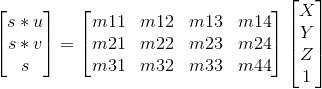
The Camera Projection Matrix (M) is the product of the intrinsic (K) matrix and the extrinsic ([R|T]) matrix. Intuitively, the matrix defines the transformation between 3D world coordinates and 2D image coordinates (where (su,sv,s) are homogenous image coordinates and (x,y,z,1) are homogenous world coordinates):
The steps to solve for M are as follows:
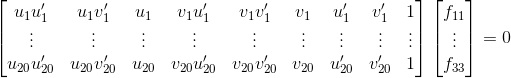
1. Gather at least 6 points pairs to create the following linear homogenous system (Note that we are given 20 points to use, so I include all 20 in the system):

2. Take the SVD of the leftmost matrix above (notice that the equation above takes the form of Ax=0. A solution for x can be gotten by taking the SVD of A)
3. In Matlab, SVD of A returns 3 matrices, U (Left signular vectors), S (Singular values), and V (Right singular vectors). A nx1 representation of the M matrix we are trying to solve for is found as the right-most column vector of the V matrix. So this step amounts to segmenting out that column, and reshaping it into the expected 3x4 size.
4. Now that M is solved for, the last thing to do is to solve for the camera center. If we view M as a 3x3 matrix Q appended to a 3x1 vector m4, we can easily get the camera center in one step:

Results
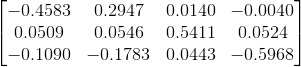
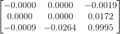
Using the pts2d-norm-pic_a.txt and pts3d-norm.txt, my camera projection matrix (M) is as follows:
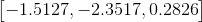
Using the same datasets, my resultant camera center is as follows:
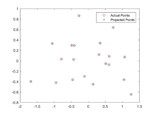
Using the estimated camera projection matrix to project the 3d points, I also compared my projection with the ground truth 2d image points. As the plot below suggests, my estimated camera projection matrix is quite accurate in this case:
Task 2: Estimate the fundamental matrix given a set of corresponding 2D points from 2 images
Epipolar geometry is the intrinsic geometry between views. The fundamental matrix (F) encapsulates this geometry. In particular, given two matching points (x and x') from the two views, the following property is satisfied:
Additionally, F can be used to find the epipolar lines corresponding to each of the points x' and x in either image:
 ,
,
 correspond to the epipolar lines associated with x' and x
respectively.
correspond to the epipolar lines associated with x' and x
respectively.
Methodology
One method to solve for F (the normalized 8-point method/the method I used), given 2 sets of corresponding points (P' and P), can be described as follows:
1. Gather at least 8 correspondances that will be needed to solve for F (Note that we are given 20 correspondances to use, so I use all 20)
2. Bells & Whistles Work - Once we have the two sets of points, we then 'normalize' both sets. This normalization consists of centering (de-meaning) each point at (0,0), and then rescaling the points such that the average squared distance from the origin is 2. Note that normalization is done separately on each set of points. This step is done to ensure good numerical conditioning. Essentially, we are going to end up taking the SVD of a matrix that contains these coordinate values, and we don't want some values in that matrix to be huge, and others to be very small (which might occur with raw coordinates).
3. Set up the following system of homogenous linear equations for F (where u',v',1 correspond to P' and u,v,1 correspond to P):
4. Similar to task 1, we again have a linear equation of the form Af = 0. So this step consists of solving for F using an SVD of A (the left-most matrix in the eq. above)
5. Enforce the singularity constraint on the F matrix. The Fundamental Matrix we currently have an estimate for is of full rank, but it is defined as a rank 2 matrix. To reduce its rank, we take the SVD of F, set it smallest singular value (in the S matrix returned from Matlab) to zero, and then reconstruct F
6. Bells & Whistles Work - Note that the Fundamental Matrix that we have estimated at this point corresponds to our 'normalized' coordinates. For this Fundamental Matrix to apply to original coordinates, I need to adjust it based on the transformations I used. The adjustment is defined as follows (where T_a corresponds to the transformation for the first set of points, and T_b corresponds to that of the second set of points):
Results
Fundamental Matrix Estimates For Base Image Pair
| Without Normalization | With Normalization | Comments |
|---|---|---|
 |
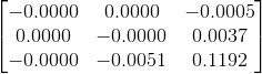 |
Admittedly, not much can be concluded from just these numerical estimates alone. I just included them here for reference. |
Fundamental Matrix Epipolar Line Evaluation
Recall from earlier that the Fundamental matrix can be used to find the epipolar
linear corresponding to x' and x. We can plot these corresponding lines against the
points they are supposed to contain to see how well the Fundamental Matrix was
estimated. This is what we do below to compare not normalizing v. normalizing:
| Normalization? | View 1 | View 2 | Comments |
|---|---|---|---|
| No | 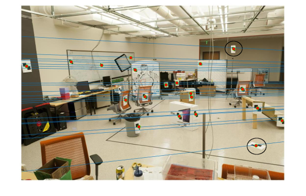 |
 |
The black circles are around instances where the epipolar lines noticeably miss the corresponding point. In general the lines are fairly close, but in some cases (particularly the 'top' black circle in both views), the line is very off. |
| Yes |  |
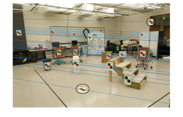 |
I've drawn black circles around the same points in this pair of images as in the previous row's pair. Clearly, the epipolar lines are better aligned to the corresponding points after including normalization (i.e. the lines go straight through the circled points instead of slightly above or slightly below). |
Task 3: Fundamental Matrix With RANSAC
For this task we are asked to use RANSAC in conjunction with Fundamental Matrix estimation from task 2 to help remove outliers from a set of possible correspondances (identified by the SIFT pipeline). The overarching idea here is that if we can calculate a geometric relationship between the two views, we can then identify and 'toss out' potential matches that don't align with this relationship.
Methodology
In particular, the steps to complete this task (and implicitly the steps that outline the RANSAC methodology) can be described as follows:
1. Randomly sample 8 distinct correspondances from the list of possible matches (recall that the minimum number of points needed for our Fundamental Matrix estimation implementation was 8)
2. Estimate a Fundamental Matrix between the two views using these 8 correspondances
3. Recall that a property of the Fundamental Matrix is that given 2 matching points x' and x:
Thus, this step amounts to calculating/storing the above quantity for every correspondance we have using the Fundamental Matrix that was just estimated.
4. Look through the stored quantities in the previous step and segment out those that fall below a certain threshold (recall that the equation above suggests that this quantity should be 0 for a match, so I chose my threshold to be something very small (0.001) in my final implementation that used normalization). The correspondances that fall below the threshold are denoted as 'inliers'.
5. Count the number of inliers that exist. If the number of inliers on this iteration is greater than on any previous iteration, save the inlier correspondances and the Fundamental Matrix that produced the outcome.
6. Repeat the above 5 steps N number of times (RANSAC is a hypothesize and test algorithm, i.e. you hypothesize and test N times and choose the best outcome from those N tries). Note that the best iteration for RANSAC would be one in which an iteration's random sample of 8 correspondances is free of any outliers. Theory suggests that the number of samples, N, needed to guarantee that this happens at least once can be described by the following equation:

'p' in the above equation is the probability that you sample at least one sample that is free of outliers, 's' is the number of points you sample each time, and 'e' is the proportion of outliers in your initial correspondance set. So given a 'p' of 99% (I'd like a 99% chance that I find at least one outlier-free sample), an 's' of 8 (this is just how we implement Fundamental Matrix Estimation), and an e of 50% (just a conservative estimate), theory suggests that I need to run the above loop 1177 times. In my actual code, I run the RANSAC hypothesize and test loop around this number of times (I run it 1000 times - I'm a little more optimistic than believing 50% of SIFT outputs are outliers).
Results
| Index | Label | Image1 | Image2 | Comments |
|---|---|---|---|---|
| 1A | Mount Rushmore Without Normalization - 225 Inliers | 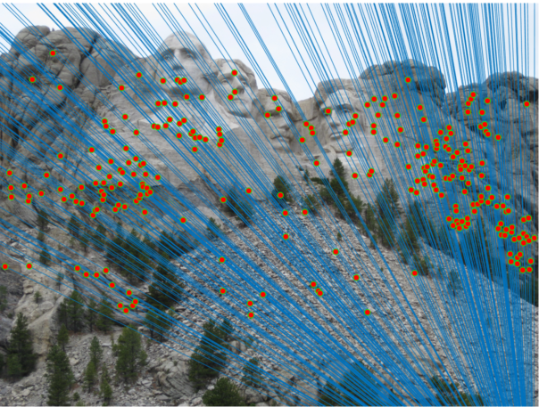 |
 |
First thing to note here is that I needed to ease my threshold for this image pair when I did not use normalization. My final implementation that includes normalization uses a thershold of 0.001 across all image sets, but to get a similar number of 'inliers' for this image set without normalization, I changed the threshold to 0.012. Having said that, the result looks pretty good - My fundamental matrix estimation results in epipolar lines that line up fairly closely to the corresponding points. Additionally, it looks like the match quality is very high (just trying to compare groups of points between the two views). It looks like for this image set, not normalizing did not have a meaningful negative impact on the result. |
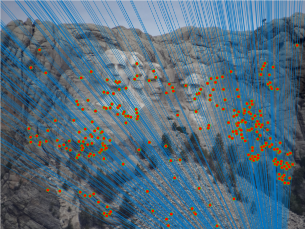
| 1B | Mount Rushmore With Normalization - 240 Inliers | 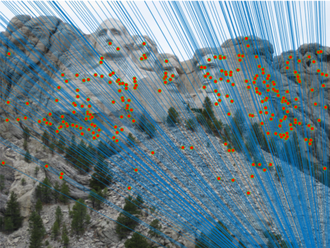 |
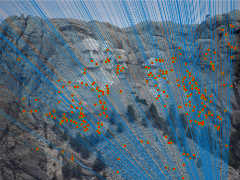 |
Using normalization on this test set (now with threshold of 0.001) produces a good result that's similar in quality to the non-normalization case above. It looks like the epipolar lines go through the corresponding points pretty accurately. Additionally, the matches across both images look almost all correct. |
| 2A | Notre Dame Without Normalization - 163 Inliers | 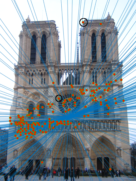 |
 |
Like image 1A, again I needed to change the threshold for the non-normalized case of the Notre Dame test set in order to get a similar number of inliers as the normalized case. More specifically I changed the threshold to 0.008 to get the result shown to the left. Note here that not normalizing seems to matter - I get a worse Fundamental Matrix estimation that results in 'mis-aligned' epipolar lines. This is shown in both images by the black circles that denote an epipolar line totally missing the corresponding point. As a result of this poor fundamental matrix estimation, you now start to see wrongful matches - note the mismatched points at the top of either tower, and some of the mismatched points on the street/behind the tree. Having said that, many of the points are still correct. |
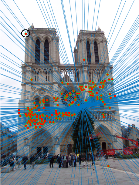
| 2B | Notre Dame With Normalization - 145 Inliers | 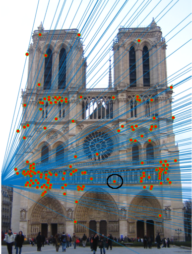 |
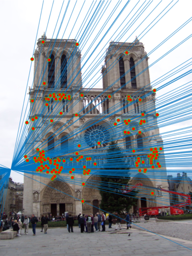 |
Including normalization seems to really fix many of the problems observed in 2A. In particular, it definitely results in better fundamental matrix estimation. This can be observed just by noticing that the epipolar lines in both views seem to really intersect the center of each point. This better estimation translates to better matches; in the two views to the left you see almost no mismatches. The only one I could find is circled in black in the left image. |
| 3A | Episcopal Gaudi Without Normalization - 120 Inliers | 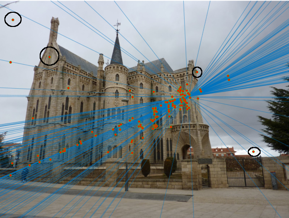 |
 |
Like the other two non-normalization results, I had to switch the threshold here as well to 0.003 to get a similar number of inliers to the normalized case. The negative effects of not normalizing are most apparent in this image test set. I've circled instances where the epipolar lines are just nowhere close to the corresponding points. This implies a poor fundamental matrix estimation and translates to many mismatches. Note that many points on the roof of the building and in the sky are matched incorrectly. In fact, many points on the left side of the building are also incorrectly matched. |
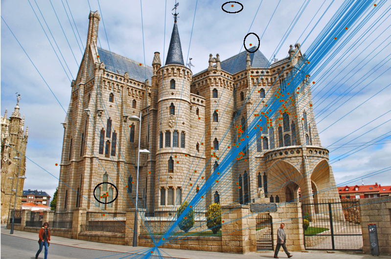
| 3B | Episcopal Gaudi With Normalization - 81 Inliers | 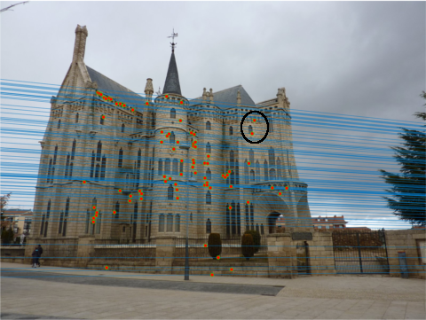 |
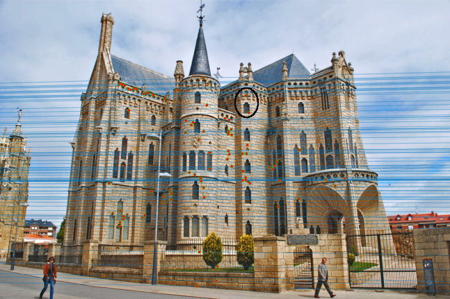 |
The advantage of including normalization is most apparent here. Unlike 3A, in this test the epipolar lines go perfectly through every point in both views. This implies a good fundamental matrix estimation and results in much fewer incorrect matches. In fact, I was only able to find two incorrect matches which have been circled in black in both views. Looking at these two incorrect matches, it's clear why they occured; the found match was on the same epipolar line and had a similar keypoint description. |