Weijian Sun

Project 3 / Camera Calibration and Fundamental Matrix Estimation with RANSAC

The goal of this project is a introduciton to camera and scene geometry. Specifically we will estimate the camera projection matrix, which maps 3D world coordinates to image coordinates, as well as the fundamental matrix, which relates points in one scene to epipolar lines in another. The camera projection matrix and the fundamental matrix can each be estimated using point correspondences. To estimate the projection matrix (camera calibration), the input is corresponding 3d and 2d points. To estimate the fundamental matrix the input is corresponding 2d points across two images. The report will start out by estimating the projection matrix and the fundamental matrix for a scene with ground truth correspondences. Then move on to estimating the fundamental matrix using point correspondences from from SIFT.

Part I: Camera Projection Matrix

The goal is to compute the projection matrix that goes from world 3D coordinates to 2D image coordinates. Recall that using homogeneous coordinates the equation for moving from 3D world to 2D camera coordinates is:

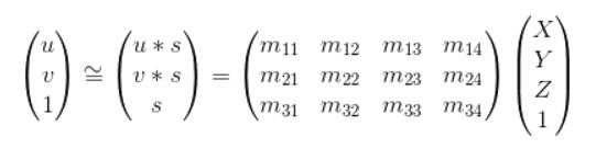
This can be writen as the following:

Here we fix the m34 to be 1 inorder to obtain a valid result via regression, then we get the following equation for n pare points:

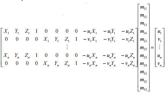
This equation can be solved by regresstion, SVD or '\' in matlab, here we impliment '\' approach and also test result with regress function in matlab.

function M = calculate_projection_matrix( Points_2D, Points_3D )

[mat1, mat2] = arrage(Points_2D, Points_3D);
%M = [regress(mat2, mat1);1];
M = [(mat1\mat2);1];
M = reshape(M, [4,3])';
end

function [mat1, mat2] = arrage(points2d, points3d)
mat1 = zeros(size(points2d,1)*2, 11);
for i=1:size(points2d, 1)
    temp = [points3d(i,:),1,zeros(1,4),-points2d(i,1)*[points3d(i,:)],;zeros(1,4),points3d(i,:),1,-points2d(i,2)*[points3d(i,:)]];
    mat1(i*2-1:i*2,:) = temp;
end
mat2 = reshape(points2d', [size(points2d,1)*size(points2d,2),1]);
end

Experiment results for part I

The total residual is: <0.0445>

The projection matrix is:

Part II: Fundamental Matrix Estimation

The second part of the project is estimating the mapping of points in one image to lines in another by means of the fundamental matrix, the definition of the Fundamental Matrix is:

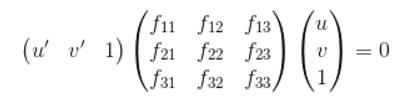
This can be writen as:

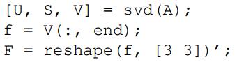
Here we solve this equation via SVD approach, that is for A*F = 0, we have:

In addition, to obtain more accuraty result, we apply normlization to the points, that is we center the image data at the origin and scale it, so the mean squared distance between the orgin and the data ppoints is 2 pixels.

More over, the least square estimate of F is full rank, however, the fundamental matrix is a rank 2 matrix. As such we must reduce its rank. In order to do this we can decompose F using singular value decomposition into the matrices U S V' = F. We can then estimate a rank 2 matrix by setting the smallest singular value in S to zero thus generating S2 . The fundamental matrix is then easily calculated as F = U S2 V'

function [ F_matrix ] = estimate_fundamental_matrix_normalized(Points_a,Points_b)

[Points_a2, Ta] = normpoint(Points_a);
[Points_b2, Tb] = normpoint(Points_b);

mat = arrage(Points_a2, Points_b2);

[U,S,V]=svd(mat);
f=V(:,end);
F=reshape(f,[3 3])';
[U, S, V] = svd(F);
S(3,3) = 0;
F_matrix2 = U*S*V';
F_matrix = Tb'*F_matrix2*Ta;

end

function [mat] = arrage(point_a, point_b)
u = point_b(:,1);
v = point_a(:,1);
u2 = point_b(:,2);
v2 = point_a(:,2);
n = size(point_a,1);
mat=[u.*v,u.*v2,u,...
    u2.*v,u2.*v2,u2,...
    v,v2,ones(n,1)];
end

function [norm, t] = normpoint(point)
means=mean(point);
Points0=point-repmat(means,[size(point, 1) 1]);
scale=1/max(max(abs(Points0)));
norm=scale*Points0;
t=[scale 0 0;0 scale 0; 0 0 1]*[1 0 -means(1);0 1 -means(2); 0 0 1];
end

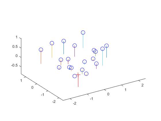
Experiment results in part II

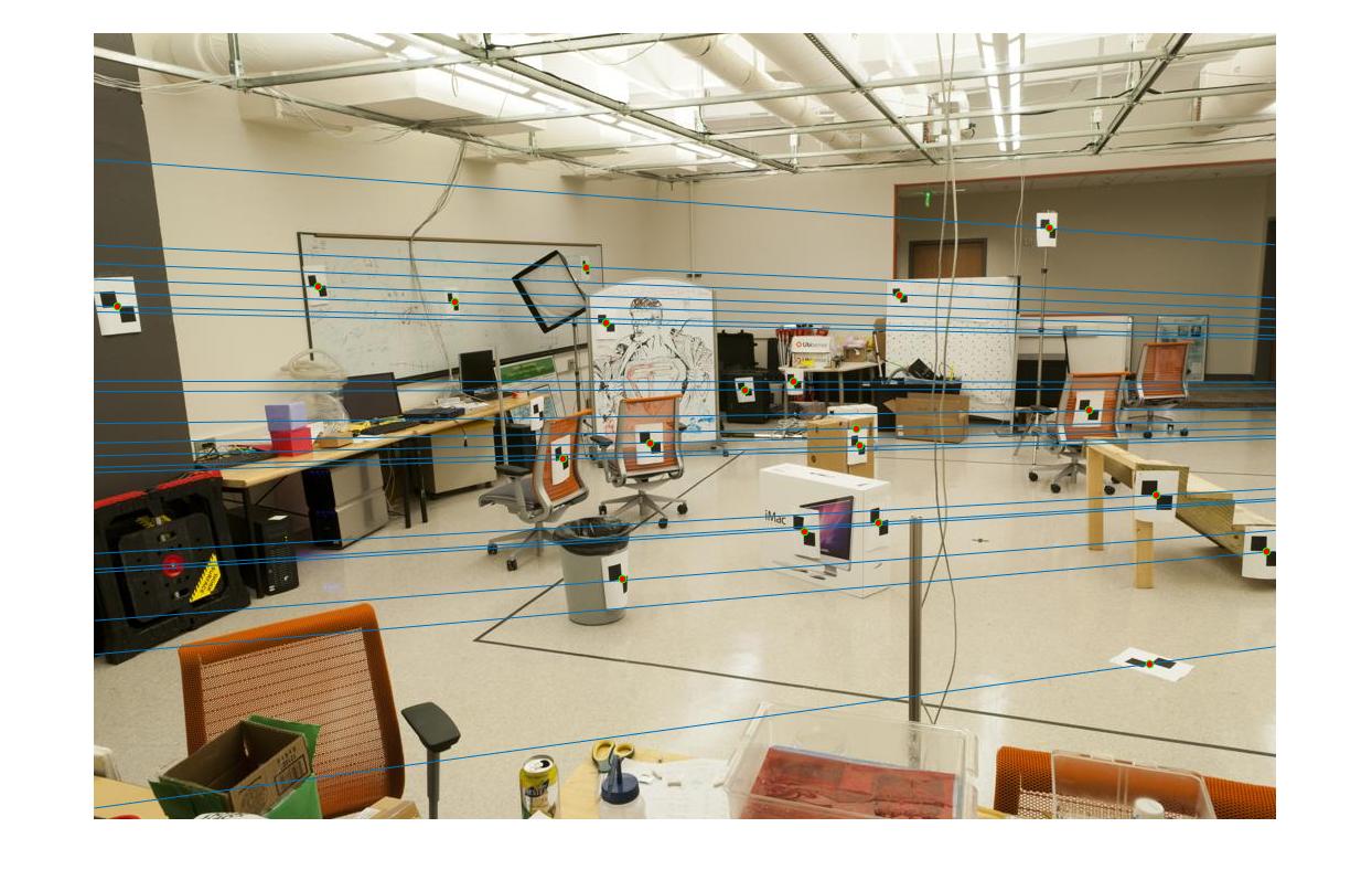
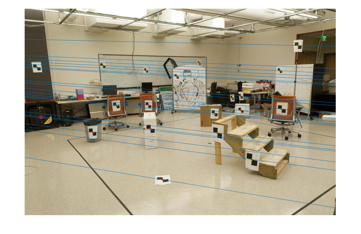
The estimated fundamantal matrix is:

We can see that all the points are dropt in the blue line, which demostratre the effective and accuraty of my algorithm, besides, the rank of the estimated matrix is 2.

Part III: Fundamental Matrix with RANSAC

In this part, i will compute the fundamental matrix with unreliable points correspondeces computed with SIFT. Under this circumstance, the least squares regression is not appropriate in this scenario due to the presence of multiple outliers. In order to estimate the fundamental matrix from this noisy data i'll use RANSAC in conjunction with fundamental matrix estimation. In RANSAC, i will iteratively choose some number of opints correspondendes, solve for the fundamental matrix using the fuction in part II, and then count the number of inliers. Inliers will be the point correspondeces that agree with the estimated fundamantal matrix. and we choose a threshold between inlier and oterlier

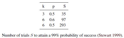
To ensure that the random sampling has a good chance of finding a true set of inliers, a sufficient number of iteration must be tried. Let p be the probability that any given correspondence is valid and P be the total probability of success after S trials. The likelihood in one trial that all k random samples are inliers is pk. Therefore, the likelihood that S such trials will all fail is

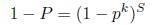
and the required minimum number of trials is

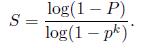
Stewart (1999) gives examples of the required number of trials S to attain a 99% probability of success. As we can see from Table, the number of trials grows quickly with the number of sample points used. This provides a strong incentive to use the minimum number of sample points k possible for any given trial, which is how RANSAC is normally used in practice.

My code is given as the following:

function [ Best_Fmatrix, inliers_a, inliers_b] = ransac_fundamental_matrix(matches_a, matches_b)

tempa = matches_a';
tempa = [tempa; ones(1,size(tempa,2))];
tempb = matches_b';
tempb = [tempb; ones(1,size(tempb,2))];

currtime = 0;
maxtime = 2000;
thredhold =0.0005
bestdis = 0;
confidence = 0.99;
bestidx = 0;
flag = 0;

while currtime < maxtime || flag ==0||size(bestidx,1)<=50

    list = randperm(size(matches_a,1));
    tempcala = tempa(:,list(1:8));
    tempcalb = tempb(:,list(1:8));

    f = estimate_fundamental_matrix(tempcala(1:2,:)', tempcalb(1:2,:)');
    
    dis = tempb' * f *tempa;
    dis = abs(diag(dis));
    
    inliersidx = find(dis<=thredhold);
    numinlier = size(inliersidx,1);
    currentdis = numinlier;%sum(dis(inliersidx))+thredhold*(size(matches_a, 1)-numinlier);
    
    if bestdis< currentdis 
        flag = 1;
        bestdis = currentdis;
        bestidx = inliersidx;
        Best_Fmatrix = f;
        ratioinlier = numinlier/size(matches_a, 1);
        num8 = ratioinlier^8;
        %uncomment this to permit self-select number of samples
        %maxtime =min(log(1-confidence)/log(1-num8), maxtime);
    end
    
    currtime = currtime +1;
end

inliers_a = matches_a(bestidx,:);
inliers_b = matches_b(bestidx,:);
end

Expriment result in part III

In this part, i have calibrate the paremeters to make the estimated resuls more accuracy. the main parameter is the least number of iteration time and the thredhold that used to judge inlier. I find that different image will correspond to different parameter to obatain more accurate estimated resuls.

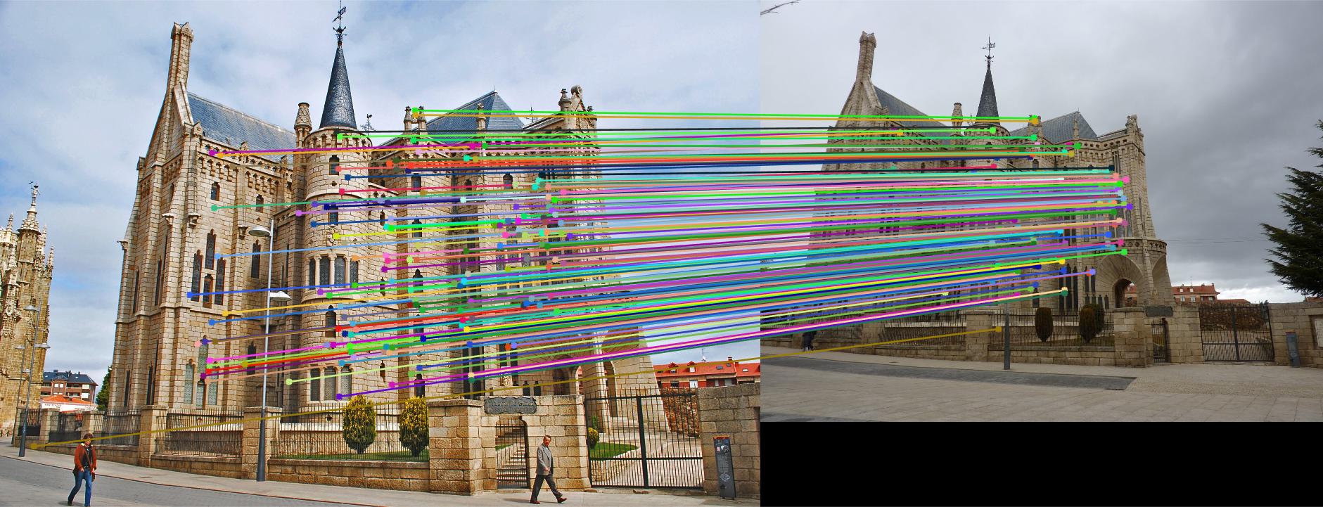
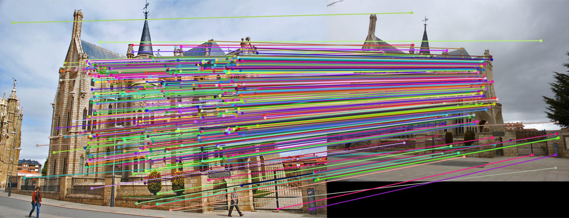
Results in Episcopal Gaudi with least number of iteration 2000 and thredhold parameter 0.0005(5*10^-4):

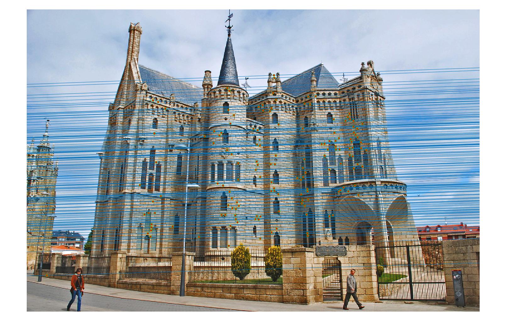
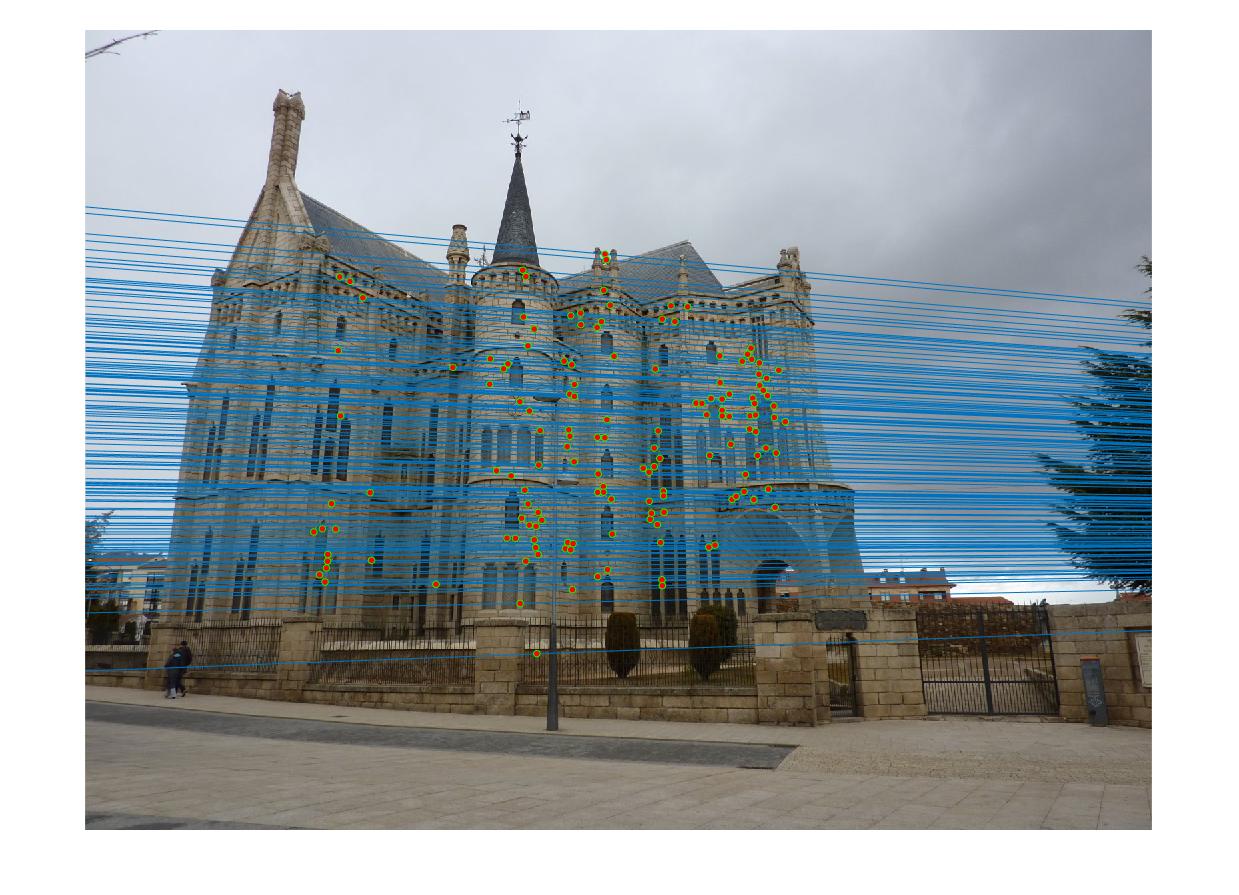
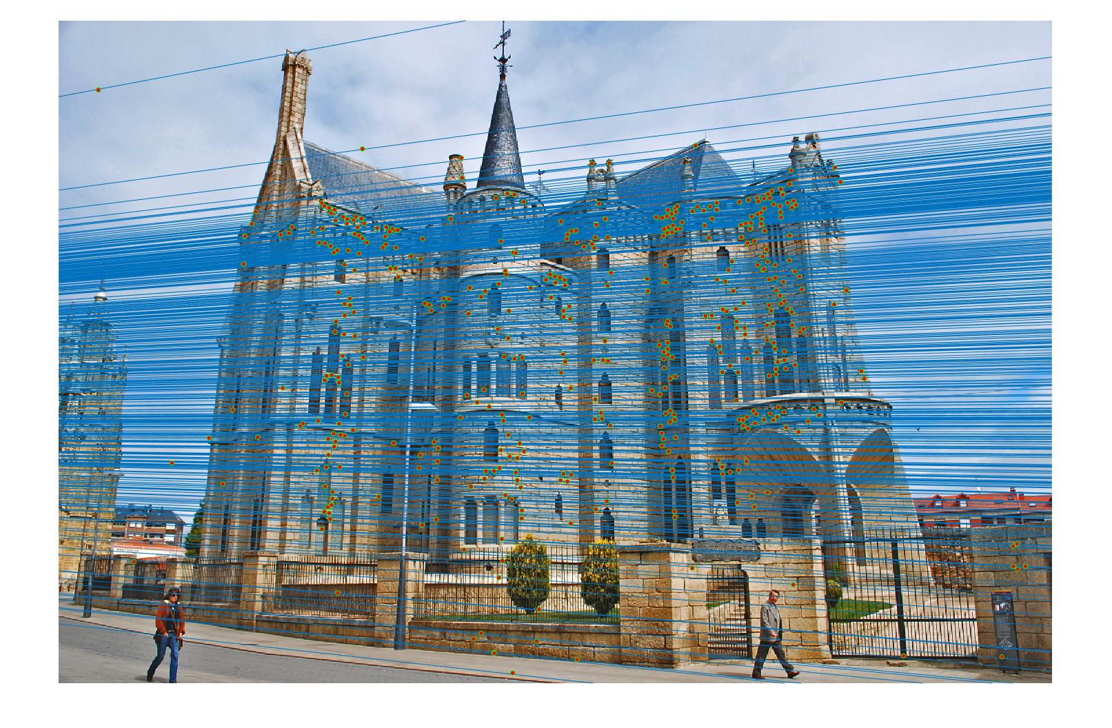
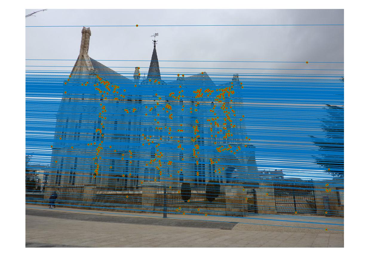
Results in Episcopal Gaudi with least number of iteration 2000 and thredhold parameter 0.005(5*10^-3):

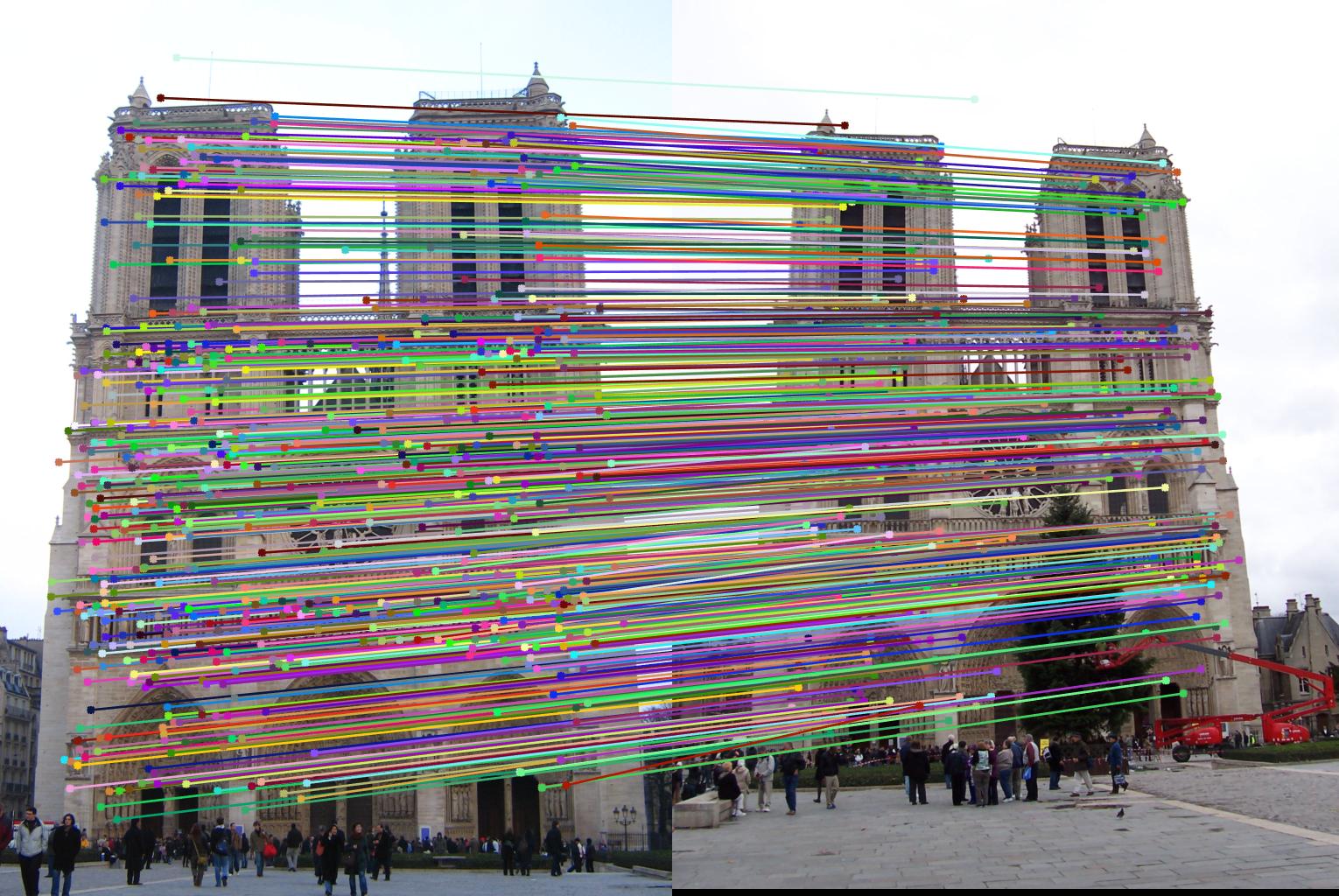
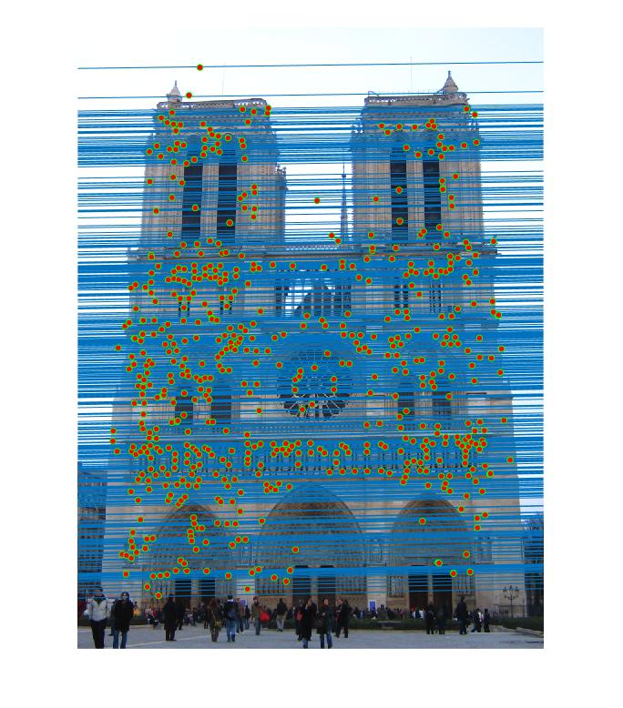
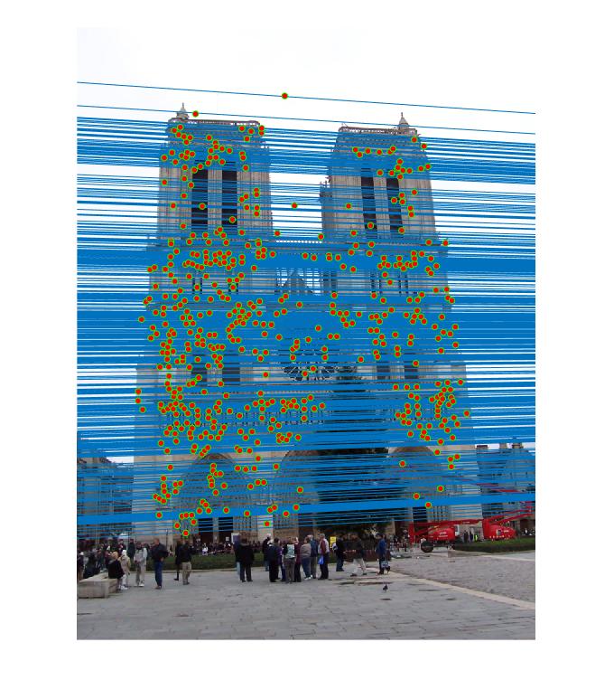
Results in Notre Dame with least number of iteration 2000 and thredhold parameter 0.005(5*10^-3):

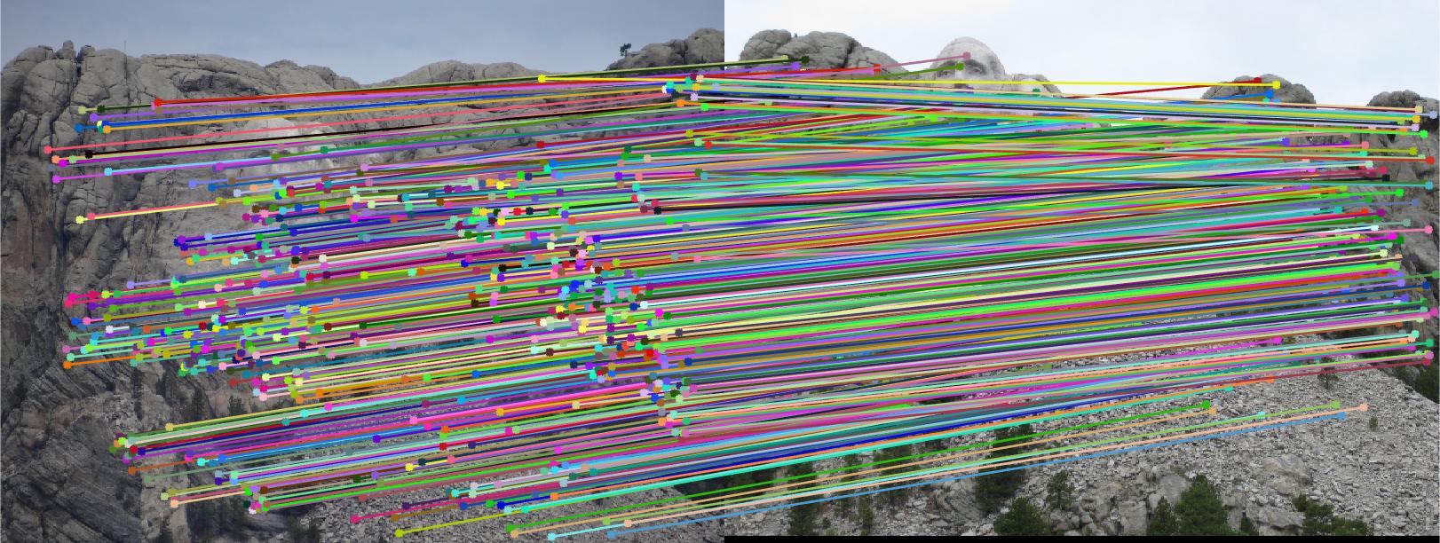
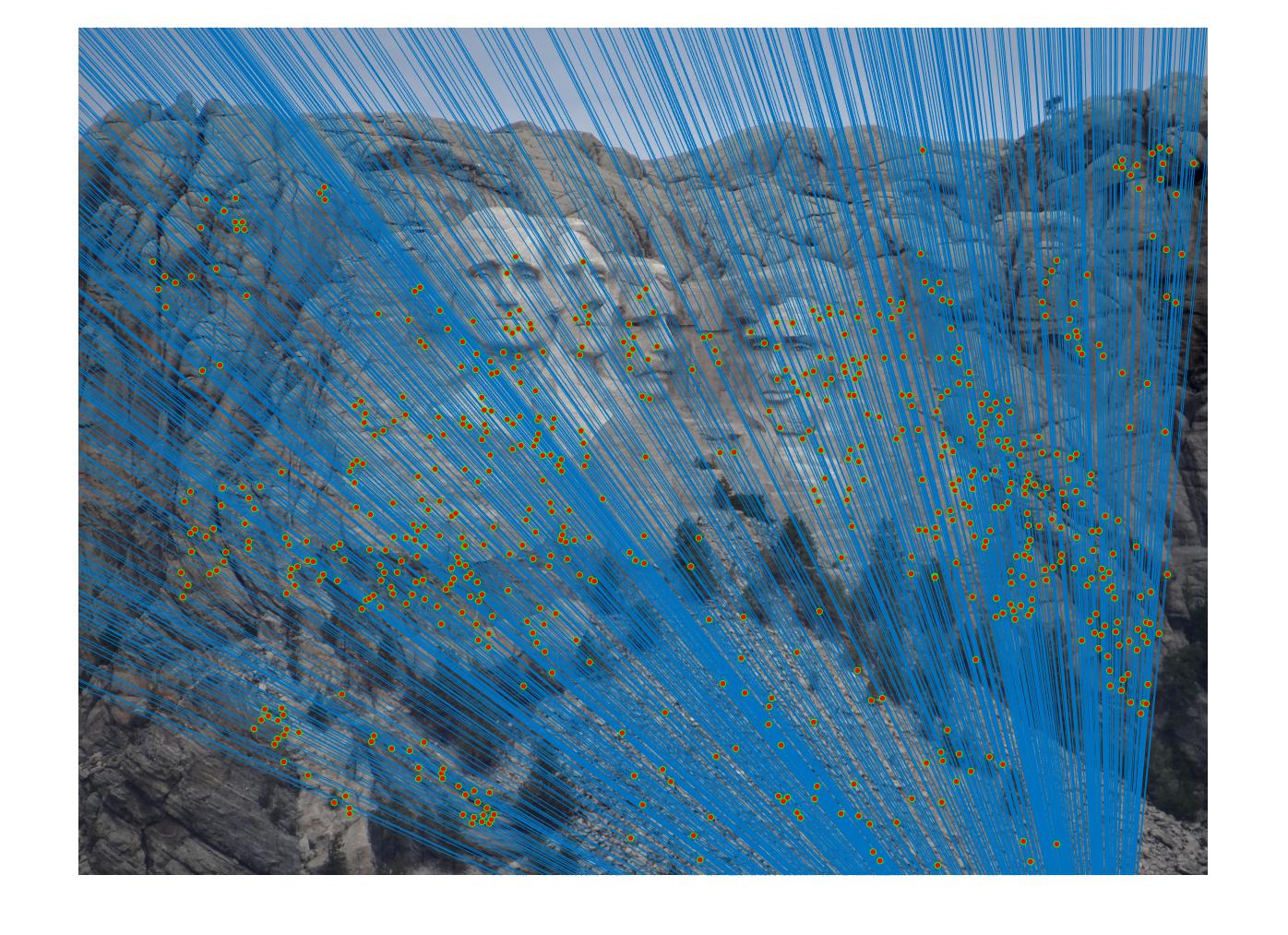
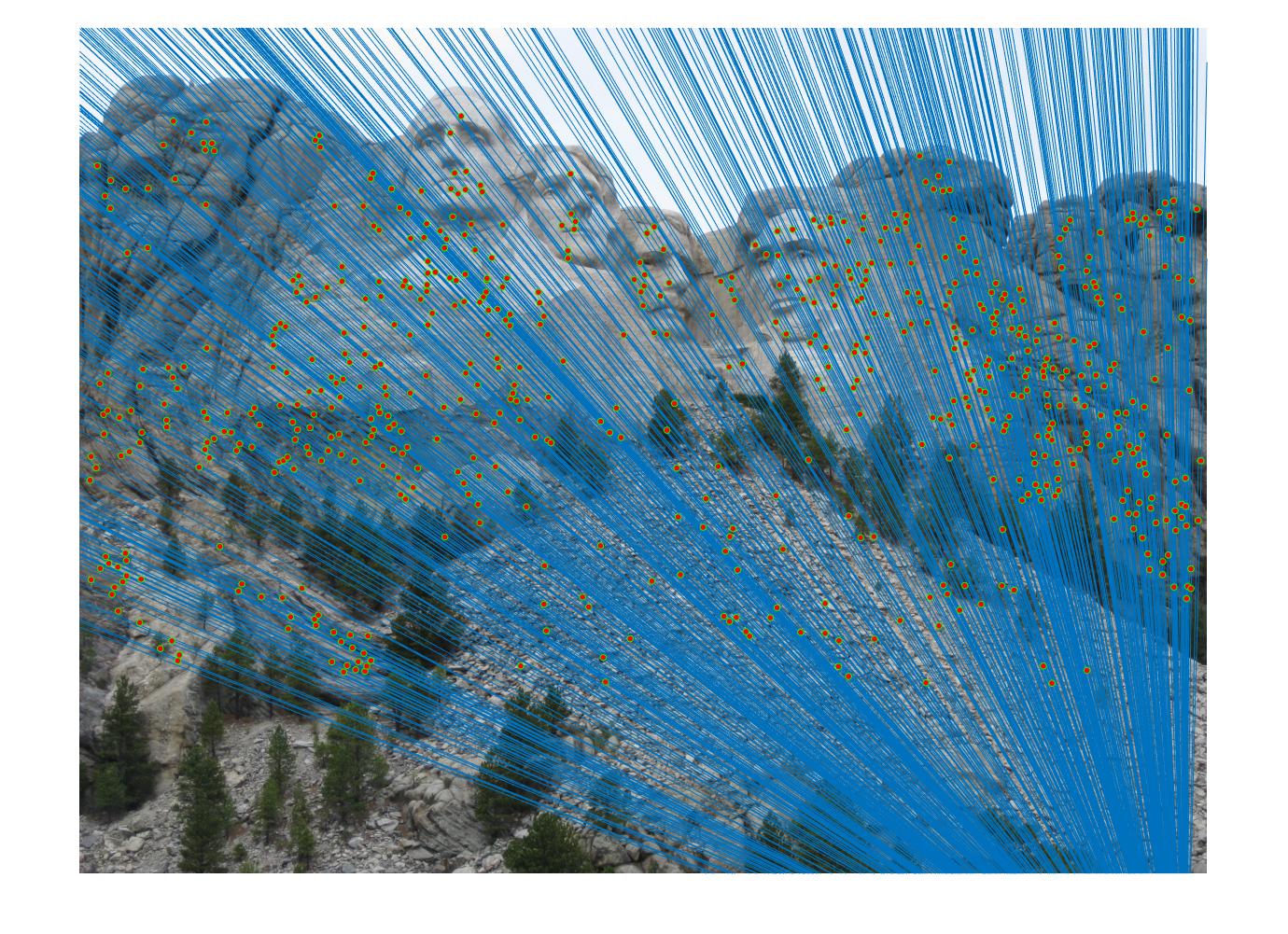
Results in Mount Rushmore with least number of iteration 2000 and thredhold parameter 0.005(5*10^-3):