Project 3 / Camera Calibration and Fundamental Matrix Estimation with RANSAC
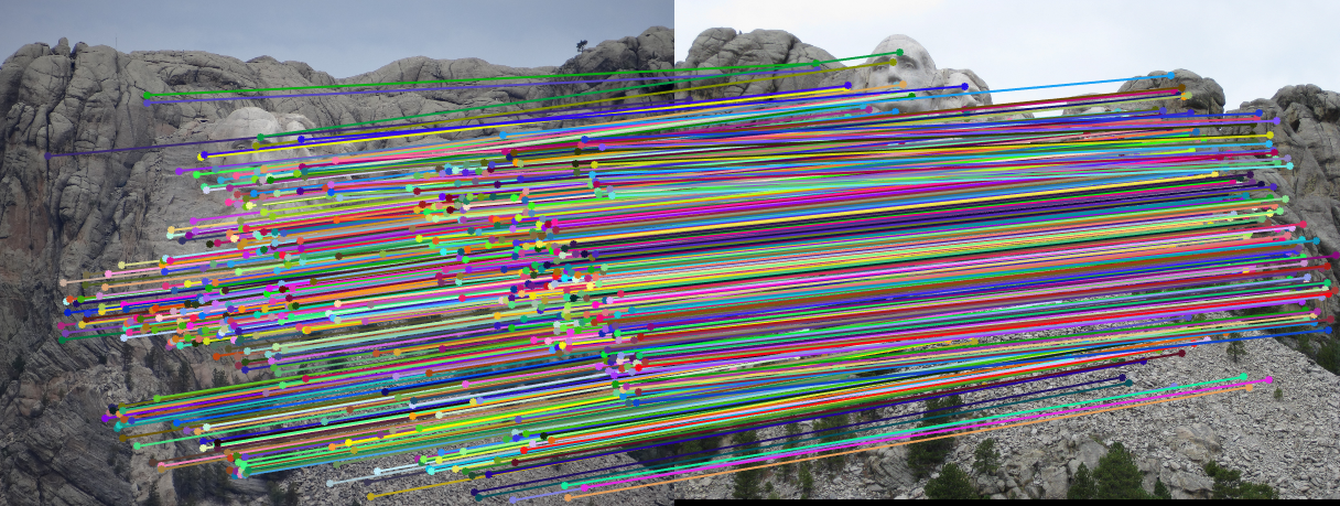
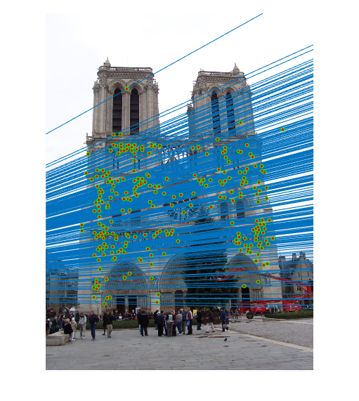
Fig.1. Example of a pair of images using RANSAC.
This project aims at introducing camera and scene geometry. In the first part, the camera projection matrix is estimated mapping the 3D coordinates to image coordinates. For the second part, the fundamental matrix is estimated and it relates the points in one figure to epipolar lines in another. RANSAC will be used to estimate fundamental matrix with unreliable SIFT matches in the third part. In the last part, I will perform normalization before computing the fundamental matrix to improve the estimation of it.
This report will discuss the project in the following portions:
- Camera Projection Matrix
- Fundamental Matrix Estimation
- Fundamental Matrix with RANSAC
- Extra Credit - Normalization
- Extra Credit - Non-normalized Data for Part 1
- Extra Credit - Another Definition for the RANSAC Threshold
- Extra Credit - Extra Images
1.Camera Projection Matrix
1.1. Algorithm
In this part, proj3_part1.m, calculate_projection_matrix.m, as well as compute_camera_center.m will be used to realize the function of computing the projection matrix from 3D to 2D coordinates and then estimating the particular extrinsic parameter - camera center in 3D world coordinates.
|
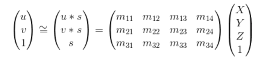
Equation.1. Equation used for moving coordinates from 3D to 2D.
The equation utilized for moving the 3D world coordinates to 2D image coordinates is shown above, where [u v 1] and [X Y Z 1] are 2D and 3D coordinates respectively. Besides, since the matrix M is only defined up to a scale, I fix the last element m34 to 1 and then the remaining coefficients will be found. The relative code is shown as follows:
    [Num] = size(Points_2D,1);

    A = zeros(Num*2, 11);
    for k = 1:1:Num
        A(2*k-1,:) = [Points_3D(k,:),1,0,0,0,0,-Points_2D(k,1)*Points_3D(k,:)];
        A(2*k,:) = [0,0,0,0,Points_3D(k,:),1,-Points_2D(k,2)*Points_3D(k,:)];
    end

    b = reshape(Points_2D',1,Num*2);
    M1=[(A'*A)^(-1)*A'*b';1];
    M=zeros(3,4);
    for n = 1:1:3
        M(n,:)=M1(4*(n-1)+1:4*n);
    end
Then, for the portion of estimating the particular extrinsic parameter - camera center in world coordinates, the following equation will be used and the corresponding code is also displayed below.
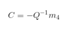
|
Equation.2. Equation for estimating the camera center.
    Q=M(1:3,1:3);
    m_4=M(:,4);
    Center=-inv(Q)*m_4;
1.2. Results
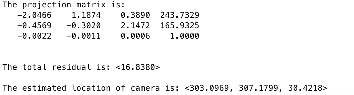
The estimated projection matrix, camera center as well as total residue is displayed below.
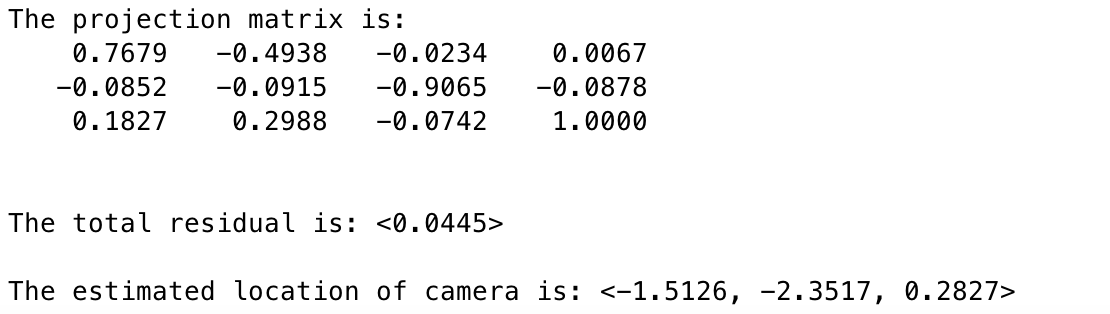
|
Fig.2. Part2 results.
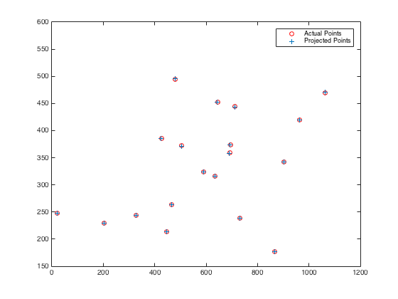
It can be easily seen that the total residual is merely 0.0445 which is very small. Compared with the given camera center which is C = <-1.5125, -2.3515, 0.2826>, the variation between the given and the estimated one is ignorable. The resulting figures are exhibited below.
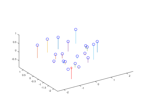
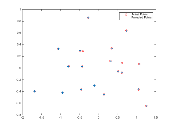
|
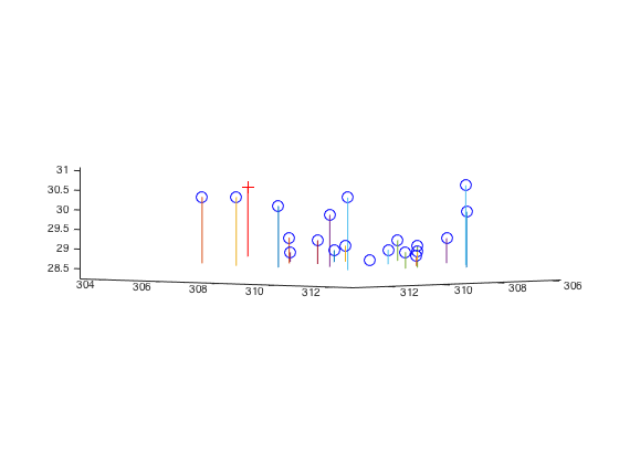
Fig.3. Camera center position. Fig.4. Actual points and projected points.
2.Fundamental Matrix Estimation
2.1. Algorithm
In this section, proj3_part2.m and estimate_fundamental_materix.m will be used. The goal of this section is to estimate the mapping of points in one image to lines in another via the use of fundamental matrix which is quite similar to the methods in the former part. The definition of the fundamental matrix is indicated as follows:
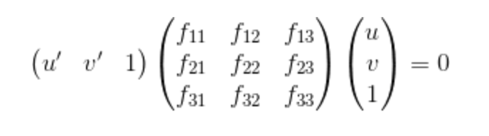
|
Equation.3. Definition of the Fundamental Matrix.
Since the fundamental matrix is a rank 2 matrix while the result of least squares estimate is full rank, F should be decomposed by using singular value decomposition (SVD) and then setting the smallest singular value in S to zero. The relative code is exhibited downwards:
    u=Points_a(:,1);
    v=Points_a(:,2);
    u1=Points_b(:,1);
    v1=Points_b(:,2);
    A = [u.*u1,v.*u1,u1,u.*v1,v.*v1,v1,u,v];
    B=ones(size(Points_a,1),1);
    f_mat=[A\(-B);1];
    f_mat = reshape(f_mat,[],3)';
    [U,S,V]=svd(f_mat);
    S(3,3)=0;
    F_matrix = U*S*V';
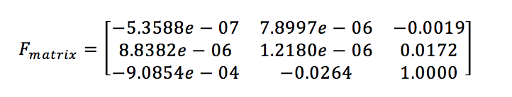
2.2. Results
The results of estimated fundamental matrix is:
|
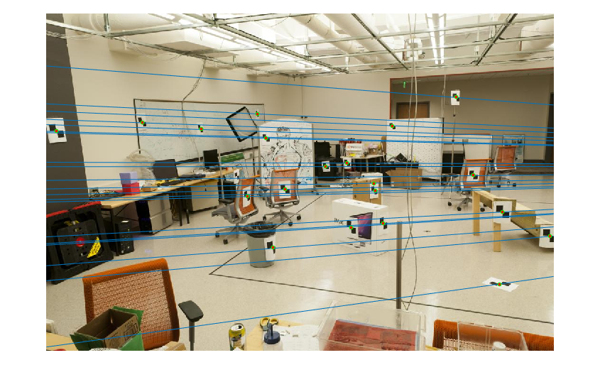
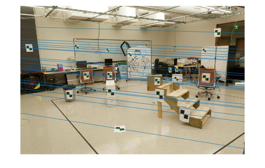
The figures with epipolar lines are shown in Fig.5. It is able to see that some epipolar lines do not exactly pass through the interest points, in other words, a little shift, which will be improved after doing normalization in part 4.

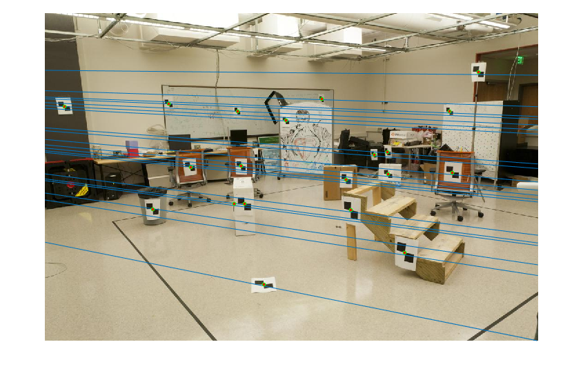
|
Fig.5. The original images with epipolar lines and interest points.
3.Fundamental Matrix with RANSAC
3.1. Algorithm
In this portion, proj3_part3.m, ransac_fundamental_matrix.m and estimate_fundamental_matrix.m will be used. Unreliable point correspondences computed with SIFT descriptors are used to estimate the fundamental matrix. RANSAC is used to enhance the accuracy by estimating the best fundamental matrix from the noisy data which means defining the inliers. The method of defining inliers is to set a threshold and if the following equations can be passed then the match is proved to be an inlier otherwise it is a outlier. In the following equation, F is the fundamental matrix and ma, mb are matching points' coordinates of two images.
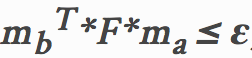
|
Equation.4. Threshold definition.
The corresponding code is as follows:
    L=size(matches_a,1);
    Num_PtCor=8;
    In_Max=0;

    for K=1:1:500
        % Randomly choose 8 numbers of point correspondences
        RandNum=randsample(L,Num_PtCor,'false');
        Fmatrix = estimate_fundamental_matrix(matches_a(RandNum,:),matches_b(RandNum,:));

        In_ID=[];
        for j=1:1:L
            ma=[matches_a(j,:) 1];
            mb=[matches_b(j,:) 1];

            threshold=0.04;
            d(j)=sum(abs(mb*Fmatrix*ma').^2)^(1/2);
            if d(j)<=threshold
                In_ID=[In_ID;j];
            end

        end

        if length(In_ID)>In_Max
            In_Max=length(In_ID);
            Best_Fmatrix=Fmatrix;
            inliers_a=matches_a(In_ID,:);
            inliers_b=matches_b(In_ID,:);

        end
    end
3.2. Results
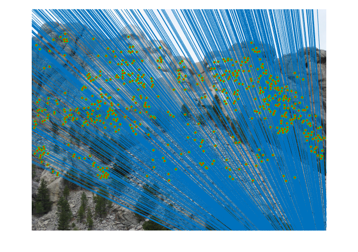
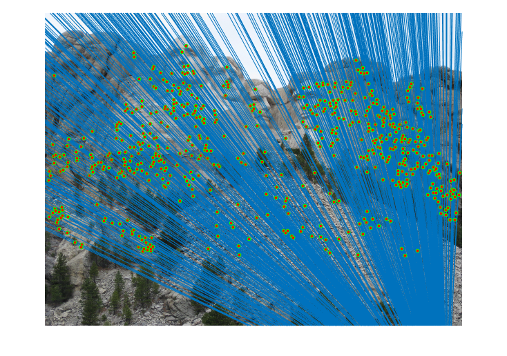
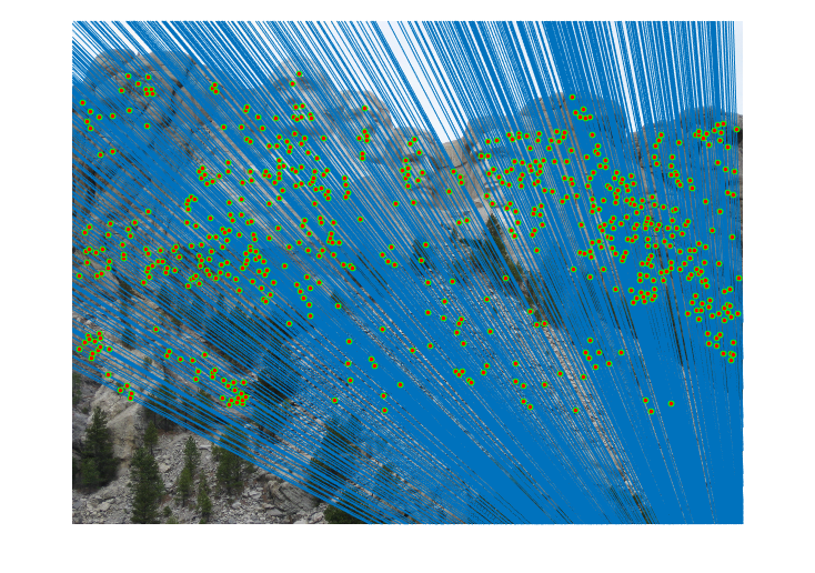
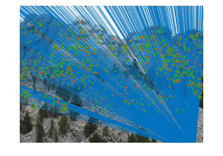
3.2.1. Mount Rushmore
|
|
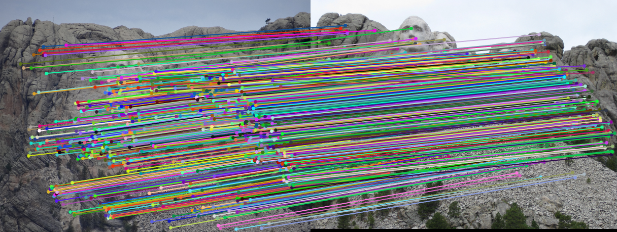
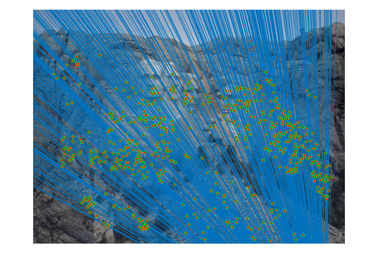
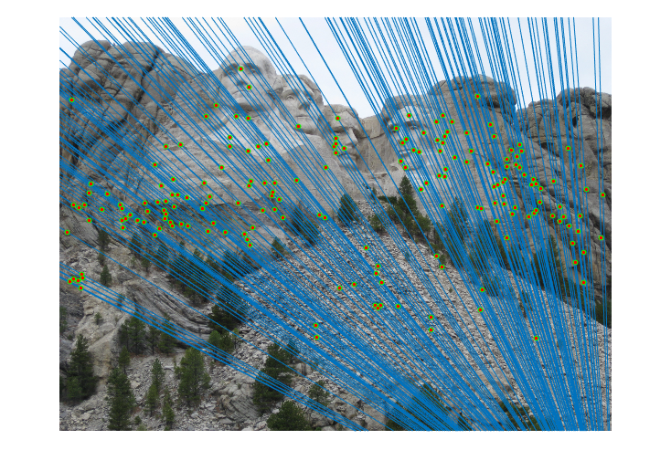
Fig.6. Results for Mount Rushmore pair of images without normalization.
The number of iterations is 500, the threshold is 0.04 and the result shows that there are 555 inliers while the total number is 825. Thus, the inlier rate is 67.27 %.
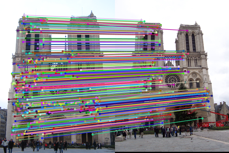
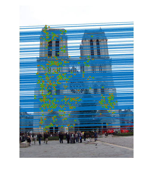
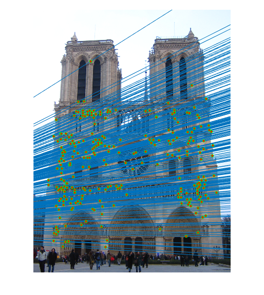
3.2.2. Notre Dame
|

|
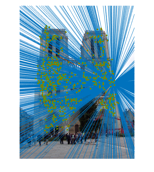
Fig.7. Results for Notre Dame pair of images without normalization.
The number of iterations is 500, the threshold is 0.03 and the result shows that there are 424 inliers while the total number is 851. Therefore, the inlier rate is 49.82 %.
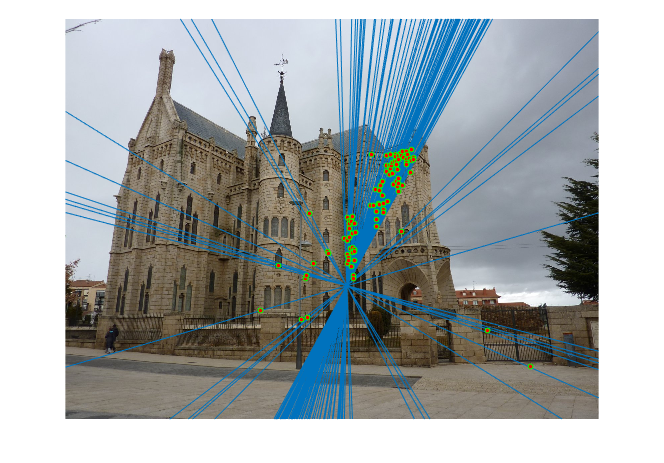
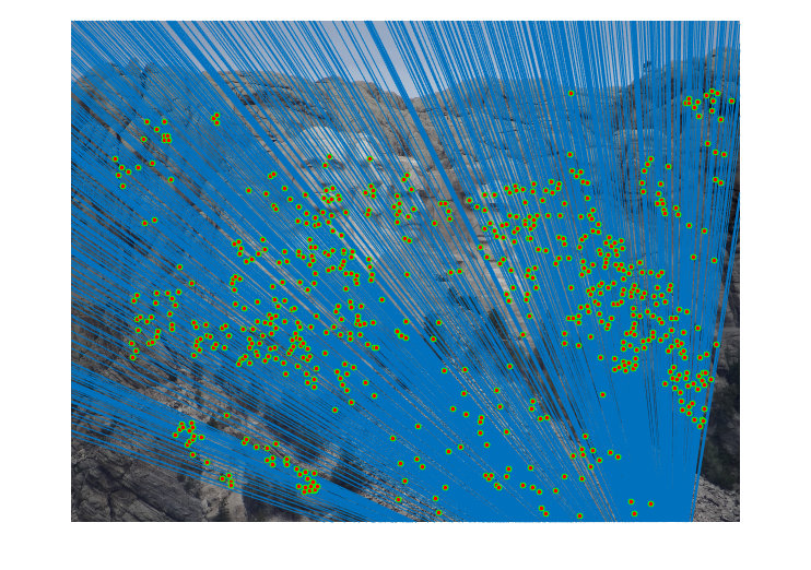
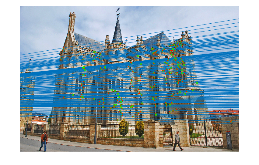
3.2.3. Episcopal Gaudi

|

|
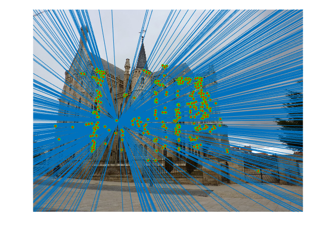
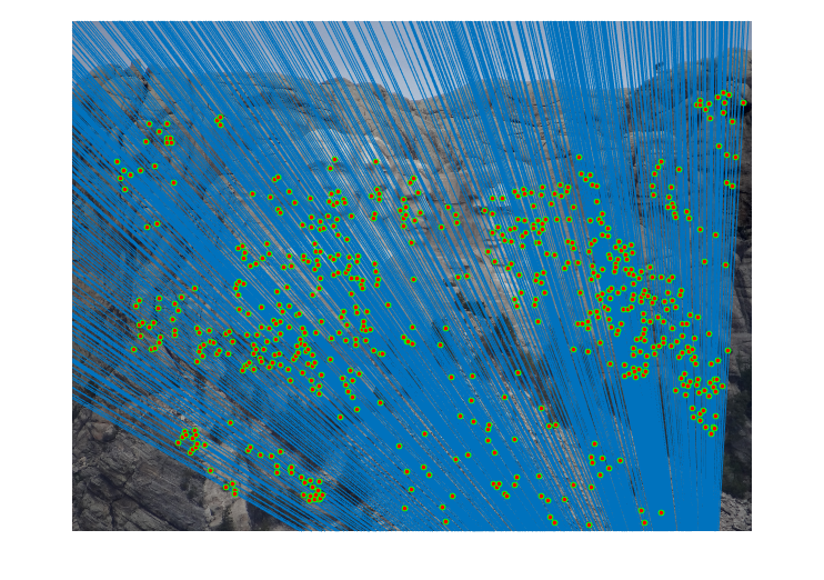
Fig.8. Results for Episcopal Gaudi pair of images without normalization.
This pair of images are quite difficult compared to the previous two and there are still some outliers showing on the figures shown above. The number of iterations is 10000, the threshold is 0.0015 and the result shows that there are 100 inliers while the total number is 1062. Consequently, the inlier rate is 9.42 %.
From the above data and figures of Episcopal Gaudi, it can be seen that the results are not quite good and the ration of inliers is quite low. Therefore, before computing the fundamental matrix, I will perform normalization of all points to improve the results.
4.Extra Credit - Normalization
4.1. Algorithm
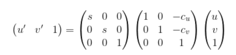
|
Equation 5. Equation for performing the normalization through linear transformations.
In this part, proj3_part3_Norm.m, ransac_fundamental_matrix_Norm.m, estimate_fundamental_matrix_Norm.m as well as Normal_Process.m will be used. The upper equation is capable of being used for performing normalization and for the parameter Cu and Cv, they are mean coordinates. For the parameter s, it is the scale factor, the reciprocal of the scale, which can be computed by estimating the standard deviation after subtracting the means. Consequently, fundamental matrix should be adjusted to operate on the original pixel coordinates. The corresponding codes are shown below:
    u=Points_a(:,1);
    u1=Points_b(:,1);
    v=Points_a(:,2);
    v1=Points_b(:,2);

    % Normalization
    [u, v, Ta] = Normal_Process(u, v, Points_a);
    [u1, v1, Tb] = Normal_Process(u1,v1,Points_b);

    % Least Square Regression
    A = [u.*u1,v.*u1,u1,u.*v1,v.*v1,v1,u,v];
    B=ones(size(Points_a,1),1);
    f_mat=[A\(-B);1];
    f_mat = reshape(f_mat,[],3)';
    [U,S,V]=svd(f_mat);
    S(3,3)=0;
    Fnorm = U*S*V';

    % Adjust fundamental matrix to operate on the original pixel coordinates.
    F_matrix=Tb'*Fnorm*Ta;
    function [ u, v, Ta ] = Normal_Process(u,v,Points_a)
    % Get Average
    avgu=sum(u)/size(Points_a,1);
    avgv=sum(v)/size(Points_a,1);
    % Substract Average
    d=((u-avgu).^2+(v-avgv).^2).^(1/2);
    % Estimate Standard Deviation
    s=std(d);
    % Normalization through Linear Transformations
    Ta=diag([1/s,1/s,1])*[1, 0, -avgu; 0, 1, -avgv; 0, 0, 1];
    PriA=Ta*([Points_a,ones(size(Points_a,1),1)]');
    u=PriA(1,:)';
    v=PriA(2,:)';
4.2. Results
4.2.1. Improved Part2 Results
|
Fig.9. The results for part2 after normalization.
Compared with the figures above and figures in part 2.2 which is without normalization, the difference seems trivial probably because the input correspondences are very perfect but it still can be seen that after normalization, the epipolar lines go more exactly through the points.
4.2.2. Improved Part3 Results - Mount Rushmore

|

|
Fig.10. Results for Mount Rushmore pair of images after normalization.
The number of iterations is 500, the threshold is 0.06 and the result shows that there are 586 inliers while the total number is 825. Thus, the inlier rate is 71.03 %.
4.2.3. Improved Part3 Results - Notre Dame

|

|
Fig.11. Results for Notre Dame pair of images after normalization.
The number of iterations is 500, the threshold is 0.05 and the result shows that there are 482 inliers while the total number is 851. Thus, the inlier rate is 58.42 %.
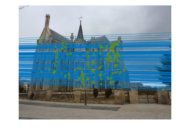
4.2.4. Improved Part3 Results - Episcopal Gaudi

|

|
Fig.12. Results for Episcopal Gaudi pair of images after normalization.
The number of iterations is 8000, the threshold is 0.055 and the result shows that there are 324 inliers while the total number is 1062. Thus, the inlier rate is 30.51 %.
It can be concluded that after doing normalization to all points, for the Mount Rushmore and the Notre Dame pairs of images, the changes of the results are not evident since the total number of inliers before and after normalization is 555 and 586 for Mount Rushmore pair of images and 424 and 482 for Notre Dame pair of images. This is probably due to the fact that most points have already been good matches and thus doing normalization will not change a lot. However, for the Episcopal Gaudi pair of images, since most points returned are not good matches, the variation is obviously for the number before and after being 145 and 324.
5.Extra Credit - Non-normalized Data for Part 1
For testing the effectiveness of the code in part 1, non-normalized data (while originally I use normalized data) is also tested. The results are shown as follows and it can be seen from the results that the residue is also small compared to the input points since the input points are much larger than normalized ones, which means the codes still work very well.
The estimated projection matrix, camera center as well as total residue utilizing non-normalized data is displayed below.
|
Fig.13. The results using non-normalized data for part 1 code.
|
Fig.14. The results for camera center position and actual as well as projected points with non-normalized data.
6.Extra Credit - Another Definition for the RANSAC Threshold
6.1. Algorithm
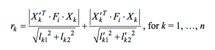
There is another method to define the threshold for selecting inliers. That is to calculate the geometrical distance between the kth match points and the corresponding epipolar lines which is defined in the following equation:
|
where

|
Equation 6. Equation for geometrical distance between the kth match points and the corresponding epipolar lines.
Thus, if the points have the geometrical distance, which is the distance between match points and the corresponding epipolar lines, within a certain value, then they are inliers otherwise they are outliers.
The corresponding code is shown as follows:
    for K=1:1:500
        % Randomly choose 8 numbers of point correspondences
        RandNum=randsample(L,Num_PtCor,'false');
        Fmatrix = estimate_fundamental_matrix_Norm(matches_a(RandNum,:),matches_b(RandNum,:));

        Lka = Fmatrix*[matches_a ones(L,1)]';
        Lkb = Fmatrix'*[matches_b ones(L,1)]';
        Xb = [matches_b ones(L,1)];
        In_ID=[];
        for j=1:1:L
            Abst = abs(Xb(j,:)*Lka(:,j));
            d(j) = Abst/sqrt(Lka(1,j).^2+Lka(2,j).^2)+ Abst/sqrt(Lkb(1,j).^2+Lkb(2,j).^2);

            if d(j) <= 0.5
                In_ID=[In_ID;j];
            end

        end

        if length(In_ID)>In_Max
            In_Max=length(In_ID);
            Best_Fmatrix=Fmatrix;
            inliers_a=matches_a(In_ID,:);
            inliers_b=matches_b(In_ID,:);
        end
    end
6.2. Results
6.2.1. Mount Rushmore
Table 1. The relationship between threshold and inlier ratio for Mount Rushmore pair of images.
| Threshold | Iterations | Inliers | Ratio (Inliers/Total) |
| 0.5 | 500 | 190 | 23.03 % |
| 5 | 500 | 641 | 77.70 % |
| 10 | 500 | 658 | 79.76 % |
| 20 | 500 | 665 | 80.61 % |
| 30 | 500 | 667 | 80.85 % |
It can be seen from the above table that with the increase of threshold value, the number of inliers also enhances but when it comes to a quite large number like 10, 20 or 30, the increment seems trivial and the outliers come into being on the figures with threshold value of 30 shown below.

|

|
Fig.15. Results for Mount Rushmore pair of images after normalization using geometric distance threshold method and the threshold value is 0.5.

|
|
Fig.16. Results for Mount Rushmore pair of images after normalization using geometric distance threshold method and the threshold value is 5.

|
|
Fig.17. Results for Mount Rushmore pair of images after normalization using geometric distance threshold method and the threshold value is 30.
6.2.2. Notre Dame

|
|
Fig.18. Results for Notre Dame pair of images after normalization using geometric distance threshold method and the threshold value is 1.
6.2.3. Episcopal Gaudi

|
|
Fig.19. Results for Episcopal Gaudi pair of images after normalization using geometric distance threshold method and the threshold value is 1.5.
7.Extra Credit - Extra Images
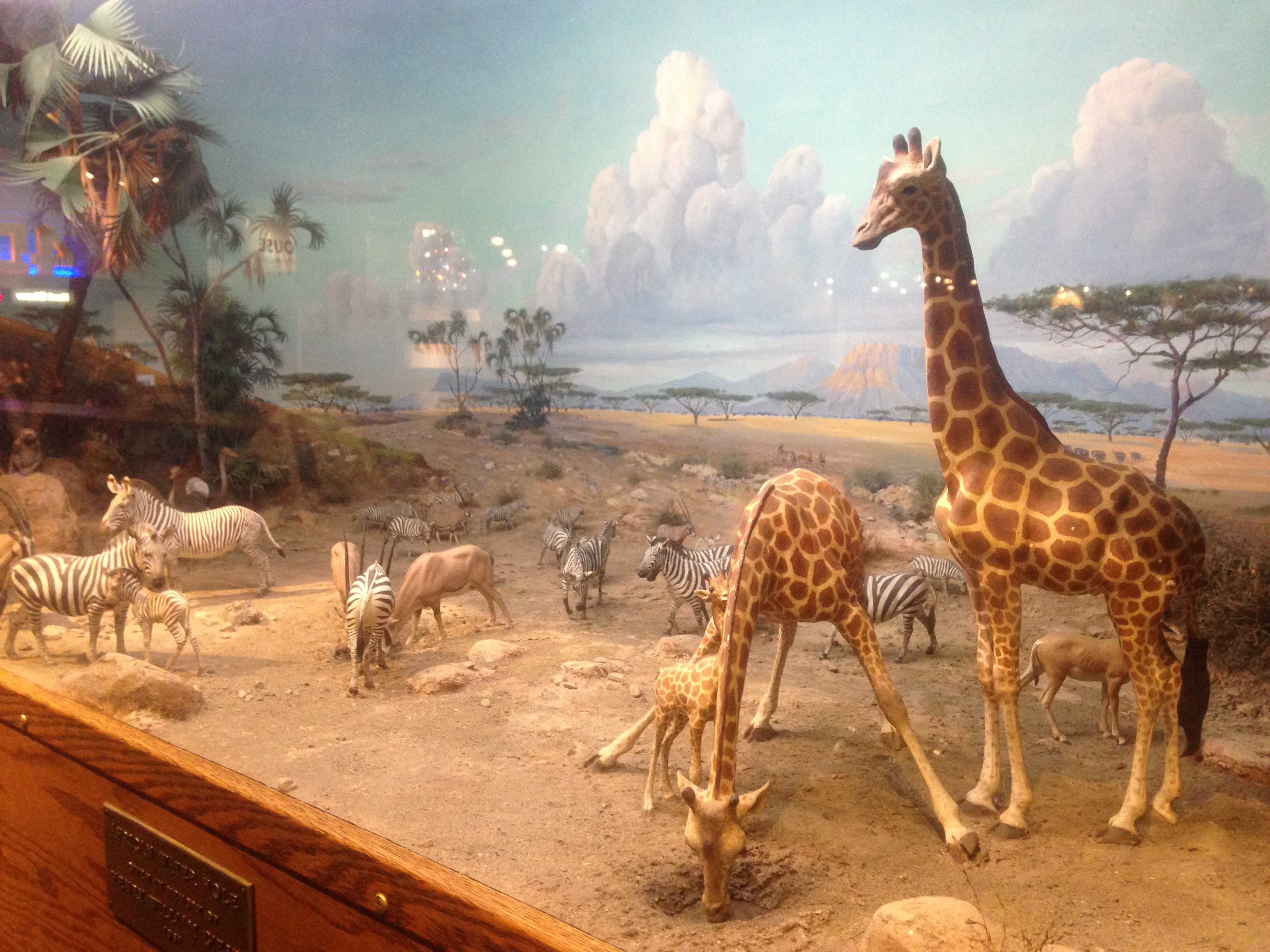
7.1. Boston Museum of Science
|

|


|
Fig.20. Results for Boston Museum of Science pair of images with normalization.

|


|
Fig.21. Results for Boston Museum of Science pair of images without normalization.
The parameters are set as follows: the iteration numbers for both case are 500; for the case with normalization, the threshold is 0.06 and the inlier number is 696 over total 764; for the case without normalization, the threshold is 0.02 and the inlier number is 712 over total 764. This pair of images shows extremely perfect matching and the ratios of inliers in both case - with and without normalization are all above 90 % probably because most points have already been good matches.
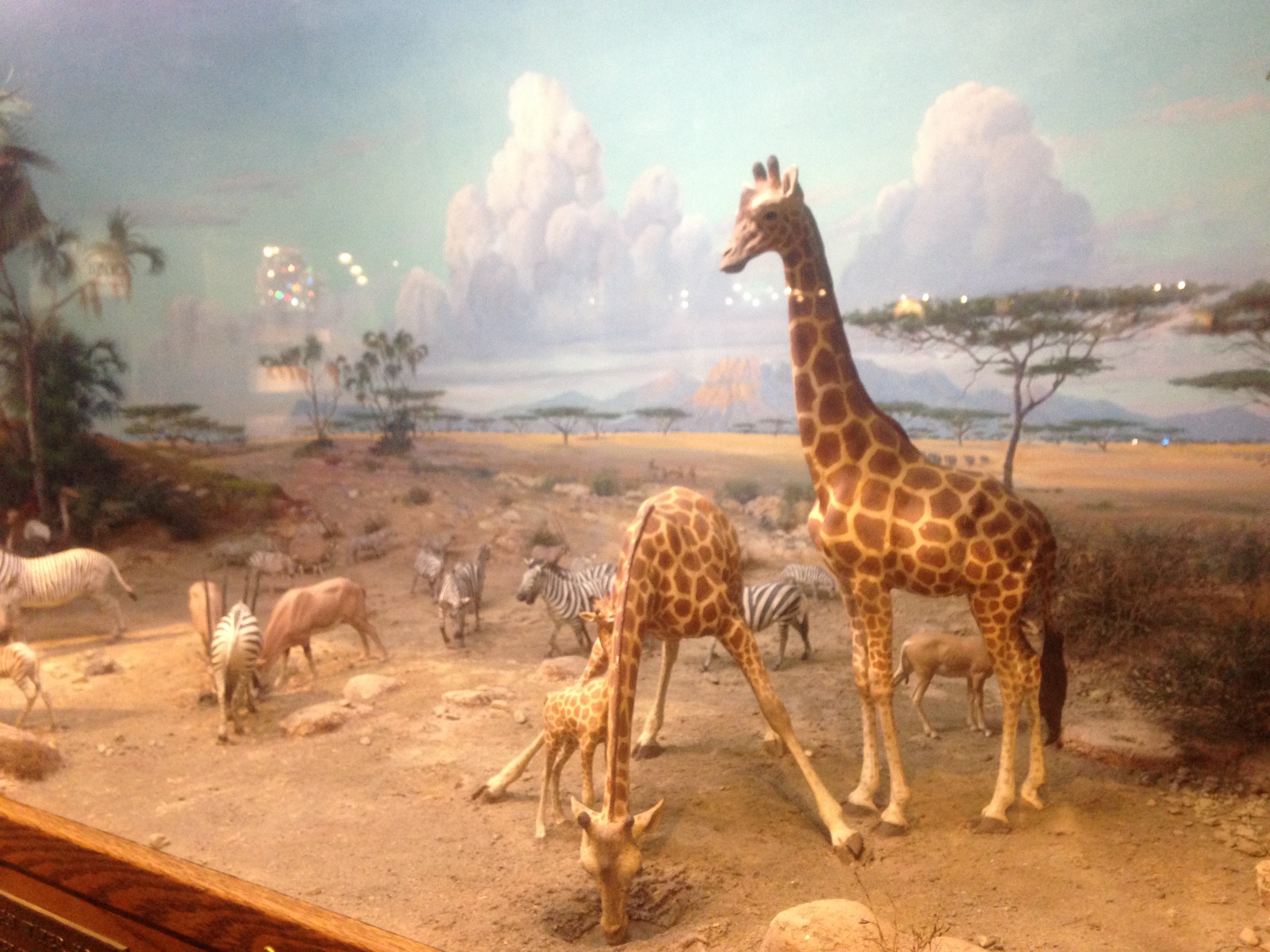
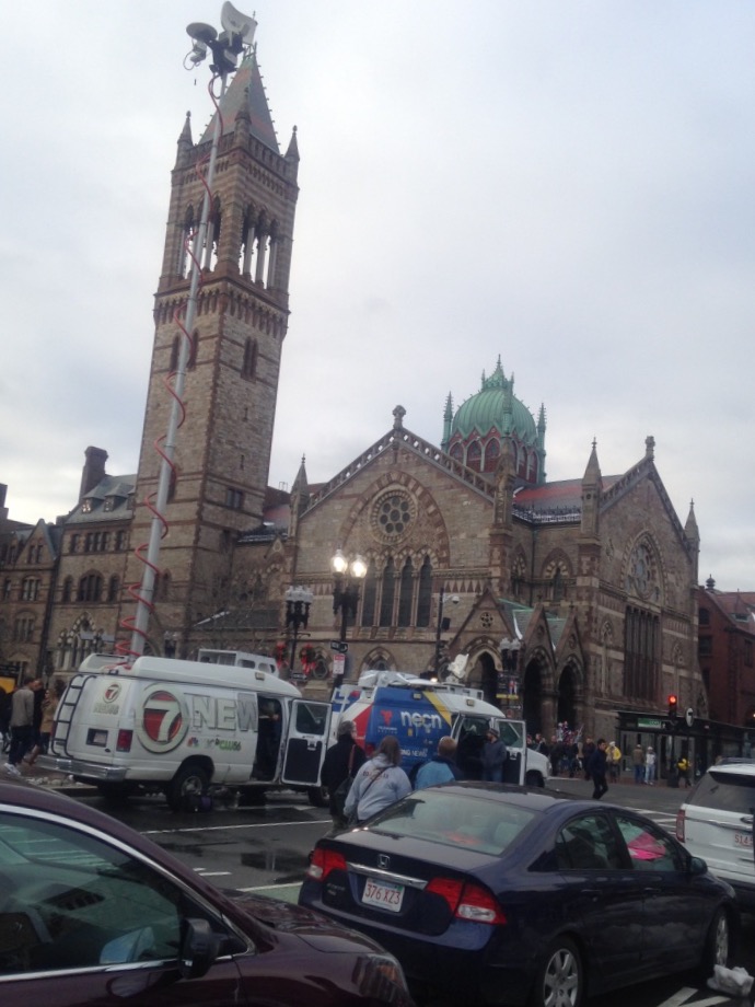
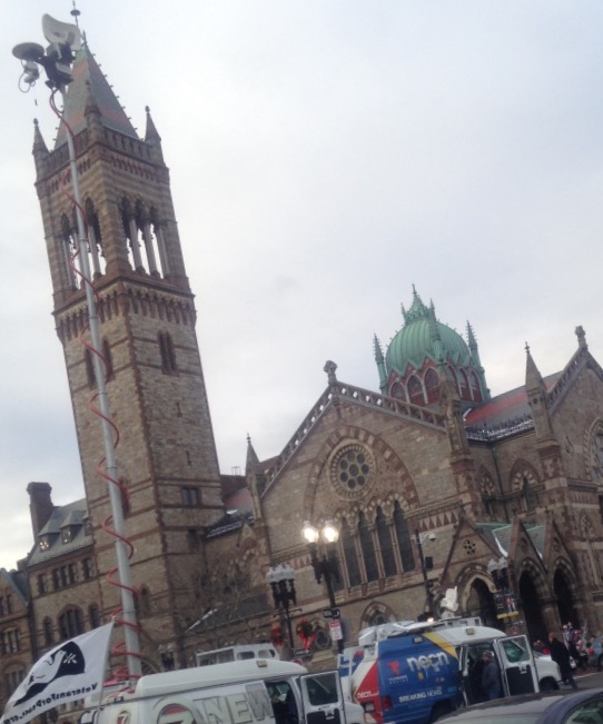
7.2. Boston New Year
|

|


|
Fig.22. Results for Boston New Year pair of images with normalization.

|


|
Fig.23. Results for Boston New Year pair of images without normalization.
For this pair of images, both the results with and without normalization have been shown above. The number of iterations are all set as 6000 and the threshold is 0.08 and 0.02 for with and without normalization respectively. The outcomes indicate that the number of inliers are 437 and 440 with the sum of inliers and outliers being 543. Thus, despite the two images being taken at different angles and different distances, the ratio of inliers is quite high which is above 80 % showing the effectiveness of the algorithms utilized in this project.