Yuxiang Liu 903109300

RANSAC fundamental matrix

Part I

To calculate the camera projection matrix, I applied the least squares regression to solve for M given the corresponding points. Here I set up the nonhomogeneous linear system to find the elements of matrix M. After getting the projection matrix, it is easy to obtain the camera center from the equation C=-Q^-1*m4 .

% code for projection matrix
b = reshape(Points_2D',[],1);
n = size(Points_3D,1);

num_cols = 11;
A = zeros(2*n,num_cols);
zero_pad = zeros(1,4);
for i = 1:n
    A(2*i-1,:) = [Points_3D(i,:),1,zero_pad,-Points_2D(i,1)*Points_3D(i,:)];
    A(2*i,:) = [zero_pad,Points_3D(i,:),1,-Points_2D(i,2)*Points_3D(i,:)];
end
M = A\b;
M = [M;1];
M = reshape(M,[],3)';

% code for camera center
Q = M(:,1:3);
m4 = M(:,end);
Center = -inv(Q) * m4;

Results

For computing projection matrix, The projection matrix was:
0.7679 -0.4938 -0.0234 0.0067
-0.0852 -0.0915 -0.9065 -0.0878
0.1827 0.2988 -0.0742 1.0000
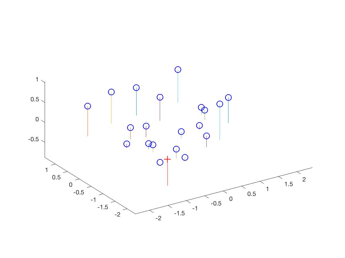
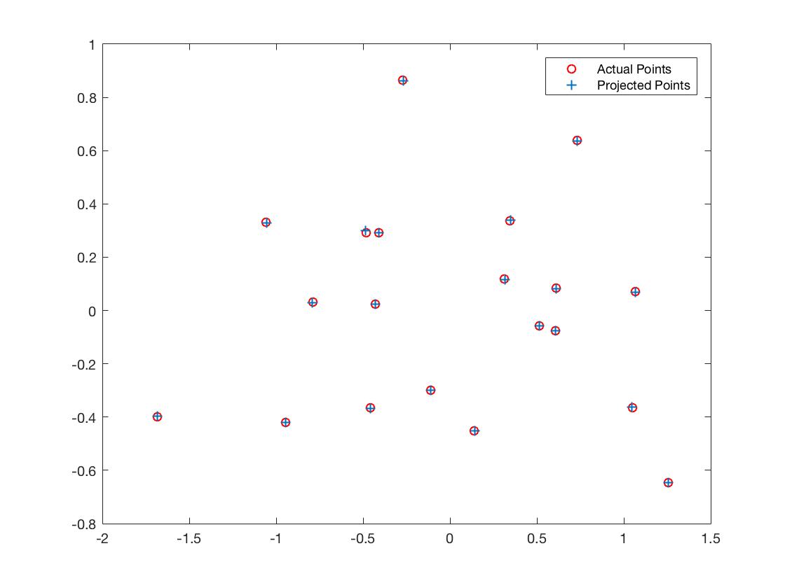
The total residual was <0.0445>, which was quite small. Finally, the estimated location of camera was <-1.5126, -2.3517, 0.2827>. It was almost the same as the expected. Meanwhile, from the chart, we can observe that match projection points quite well with the ground truth points.

Part II

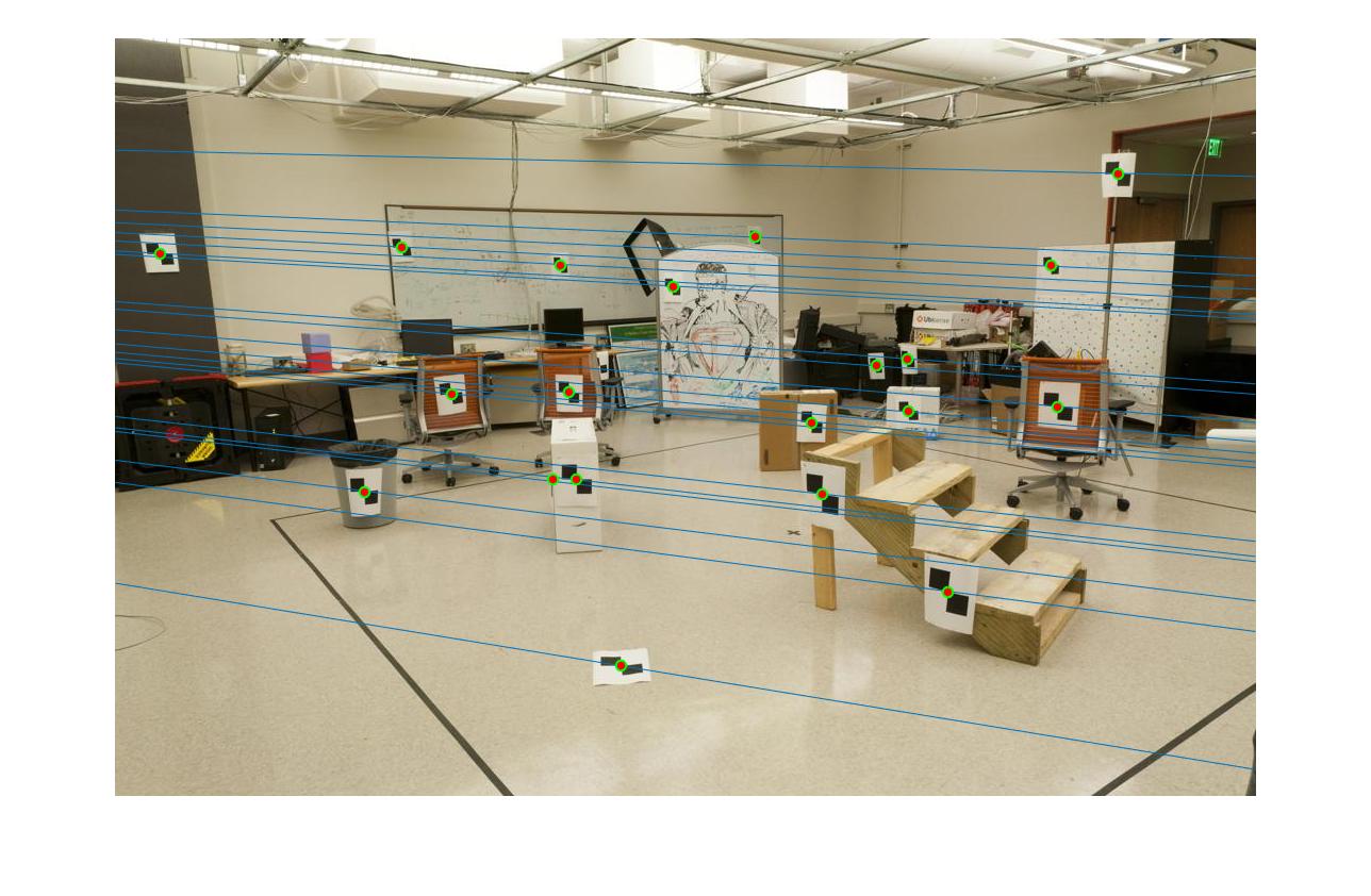
To calculate the fundamental matrix, I used a similar approach as mentioned above. First constructing the regression equation and solve it with SVD. We need to pay attention here as the fundamental matrix is a rank two matrix, which means we need to enforce the smallest singular value to be zero.

Extra Credit

For better performance, I implemented normalization when calculating the fundamental matrix. The mean of the two set of points are calculated and I substract the means to center the image data at the origin. Then I estimated the standard deviation of the points and used the reciprocal as the scale factor. After translating and scaling, we have obtained the normalized points. The actual fundamental matrix is recomputed using a formula and returned.

norm_mode = 1;
if norm_mode == 0
    n = size(Points_a,1);
    num_cols = 9;
    A = zeros(n,num_cols);

    for i = 1:n
        A(i,:) = reshape([Points_a(i,:),1]' * [Points_b(i,:),1],[1,num_cols]);
    end
    [U,S,V] = svd(A);
    f = V(:,end);
    F =reshape(f,[3,3])';

    [U, S, V] = svd(F);
    S(3,3) = 0;
    F_matrix = U*S*V';
else
    % normalization
    n = size(Points_a,1);
    num_cols = 9;
    Points_a_mean = mean(Points_a);
    Points_b_mean = mean(Points_b);
%     Points_a = bsxfun(@minus, Points_a, Points_a_mean);
%     Points_b = bsxfun(@minus, Points_b, Points_b_mean);
    Ta = [1,0,-Points_a_mean(1);
          0,1,-Points_a_mean(2);
          0,0,1];
    std_a = 1/std2(Points_a);
    Sa = [std_a,0,0;
          0,std_a,0;
          0,0,1];
    Tb = [1,0,-Points_b_mean(1);
          0,1,-Points_b_mean(2);
          0,0,1];
    std_b = 1/std2(Points_b);
    Sb = [std_b,0,0;
          0,std_b,0;
          0,0,1];
      
    Points_a = [Points_a,ones(n,1)];
    Points_b = [Points_b,ones(n,1)];
    
    Points_a_prime = (Sa * Ta * Points_a')';
    Points_b_prime = (Sb * Tb * Points_b')';
    Points_a_prime = Points_a_prime(:,1:2);
    Points_b_prime = Points_b_prime(:,1:2);
    
    
    A = zeros(n,num_cols);

    for i = 1:n
        A(i,:) = reshape([Points_a_prime(i,:),1]' * [Points_b_prime(i,:),1],[1,num_cols]);
    end
    [U,S,V] = svd(A);
    f = V(:,end);
    F =reshape(f,[3,3])';

    [U, S, V] = svd(F);
    S(3,3) = 0;
    F_matrix = U*S*V';
    
    F_matrix = (Sb*Tb)' * F_matrix * (Sa*Ta);
end

Results

Without normalization, the fundamental matrix is the following:
-0.0000 0.0000 -0.0019
0.0000 0.0000 0.0172
-0.0009 -0.0264 0.9995

With normalization, the funamental matrix turns to:
-0.0000 0.0000 -0.0003
0.0000 -0.0000 0.0027
-0.0000 -0.0037 0.0853
Since all matching points are on the corresponding epipolar lines in both cases. We are not able to observe any difference in part2 before and after normalization.

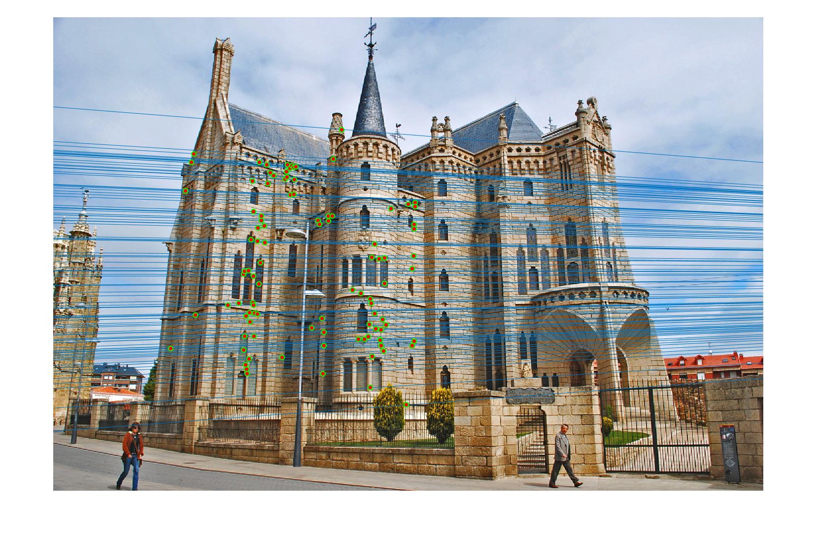
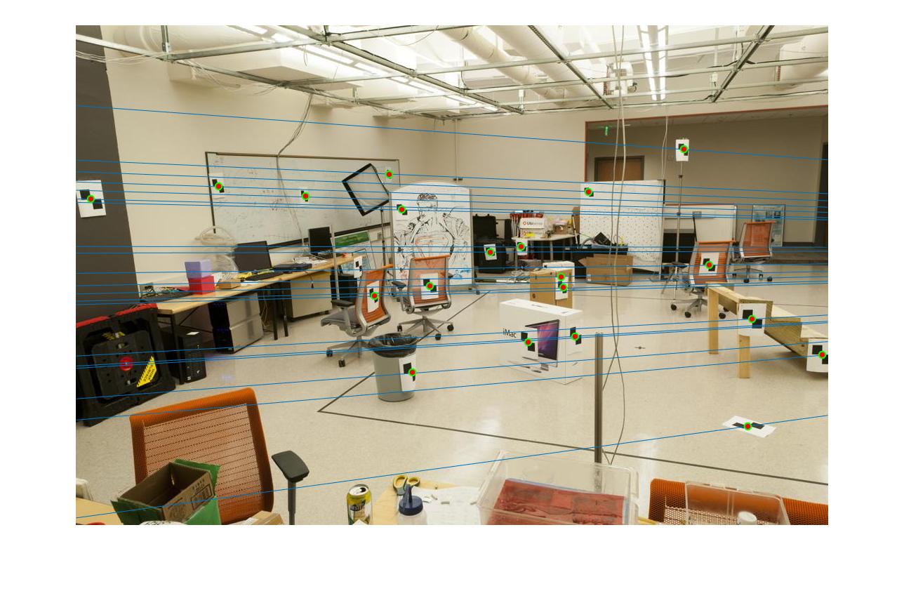
Part III

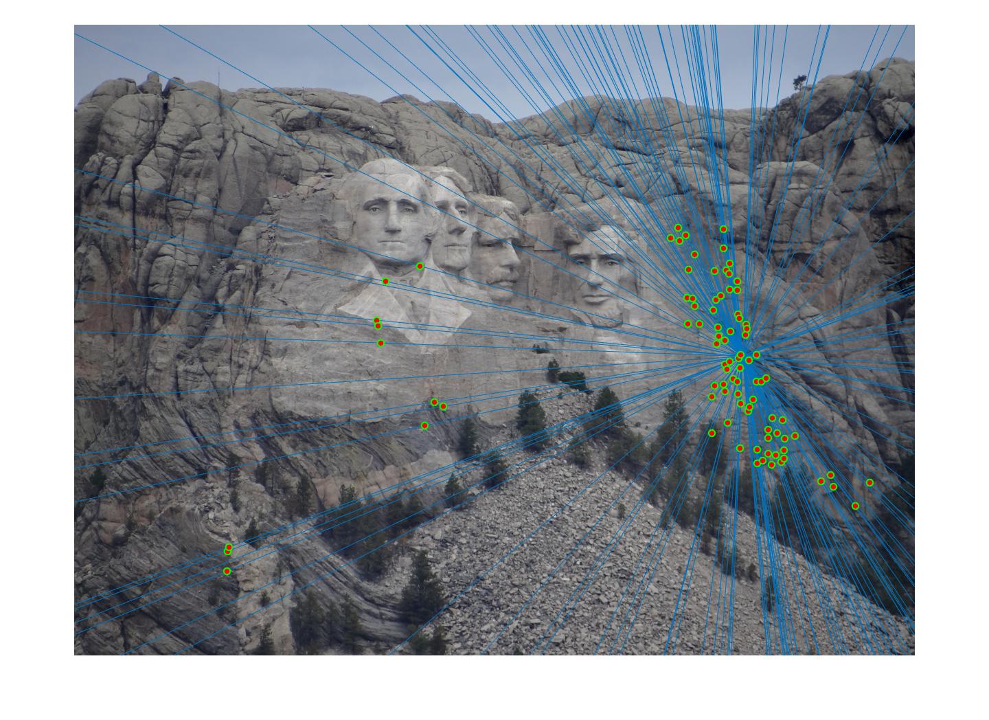
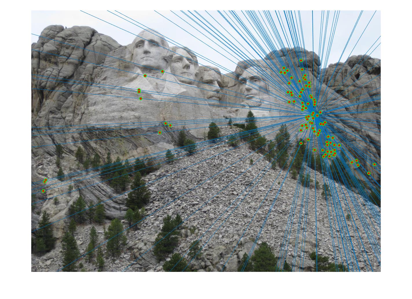
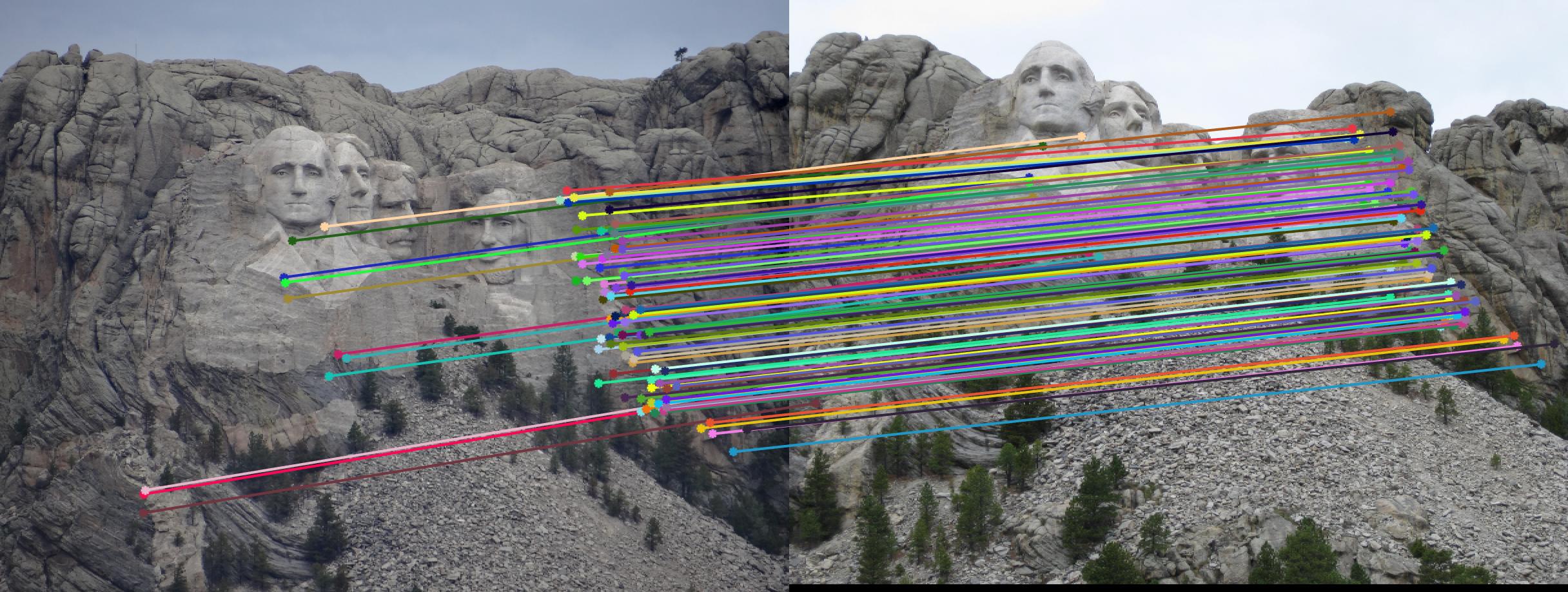
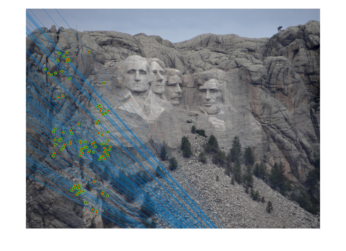
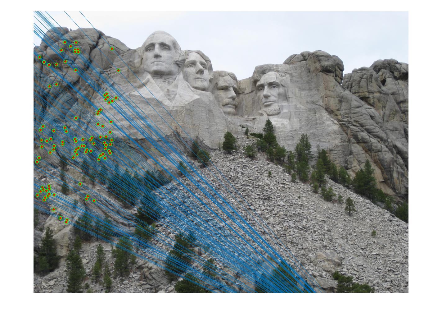
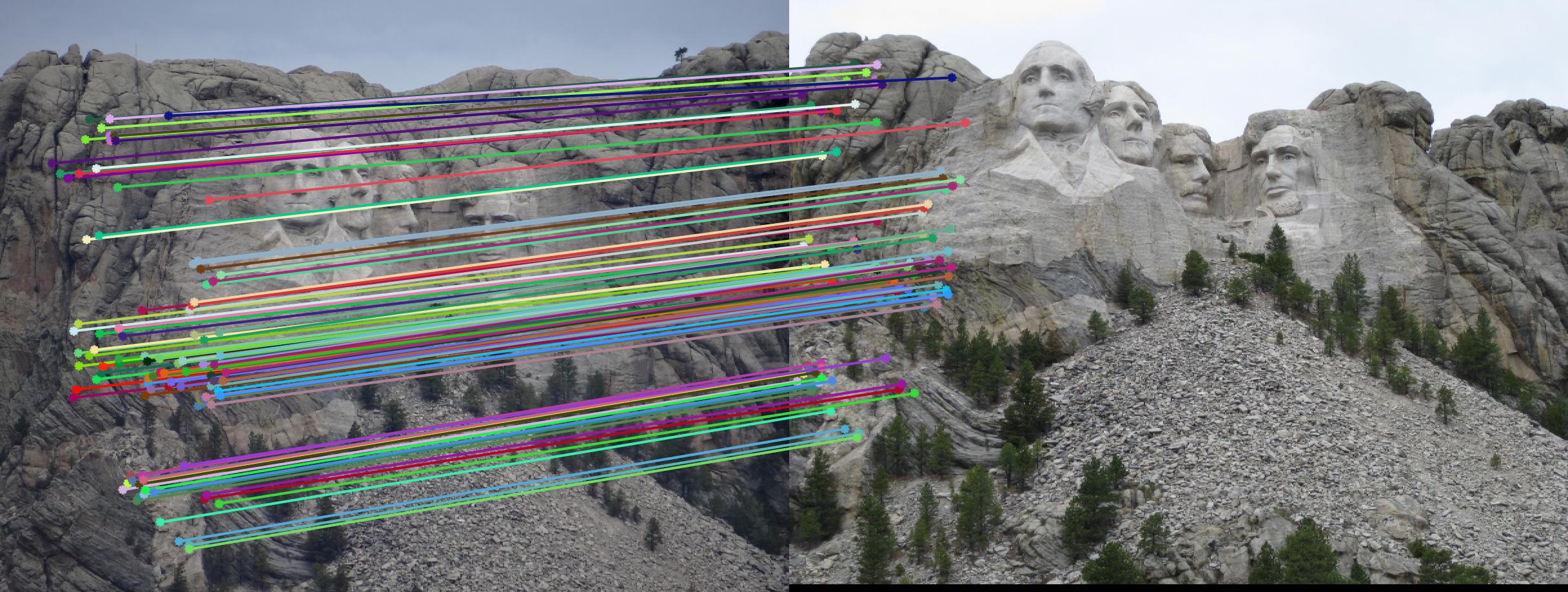
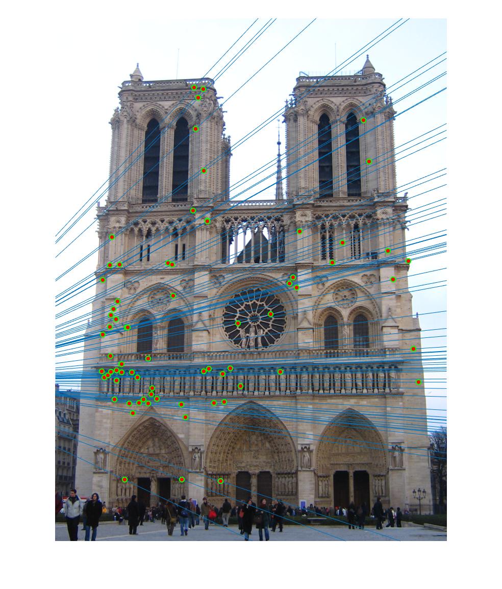
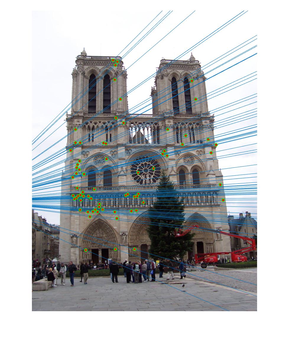
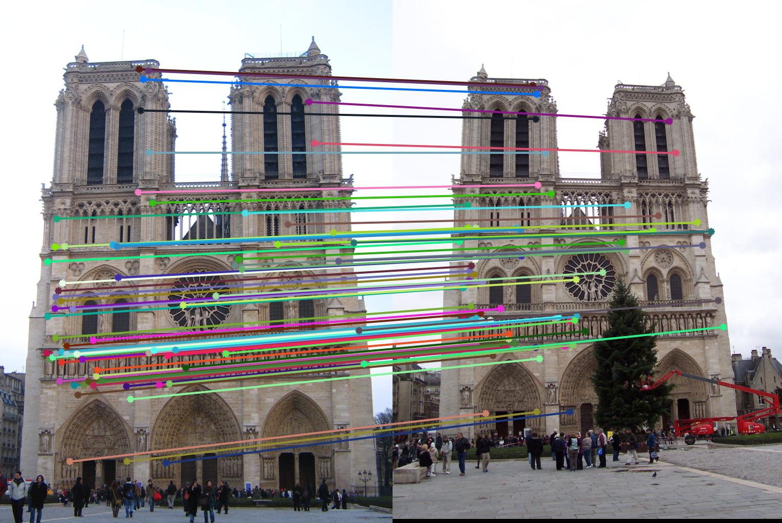
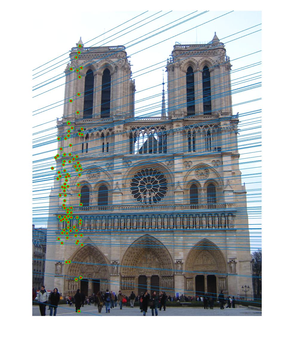
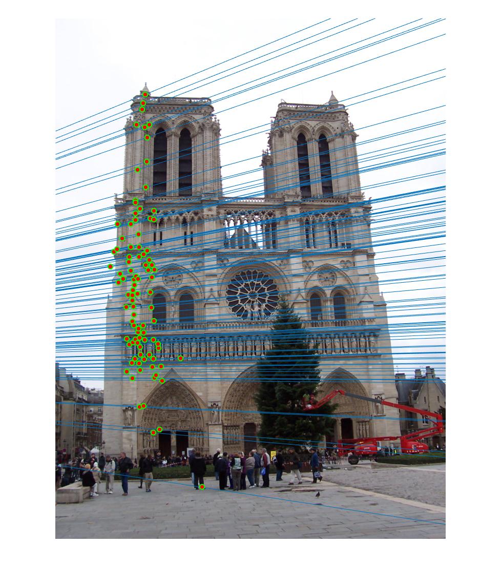
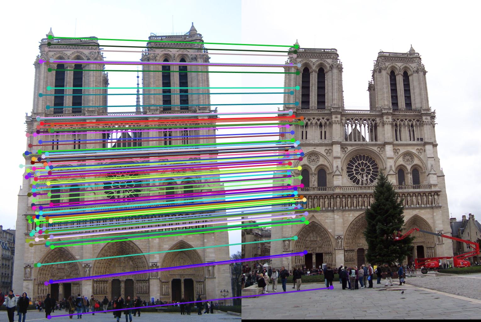
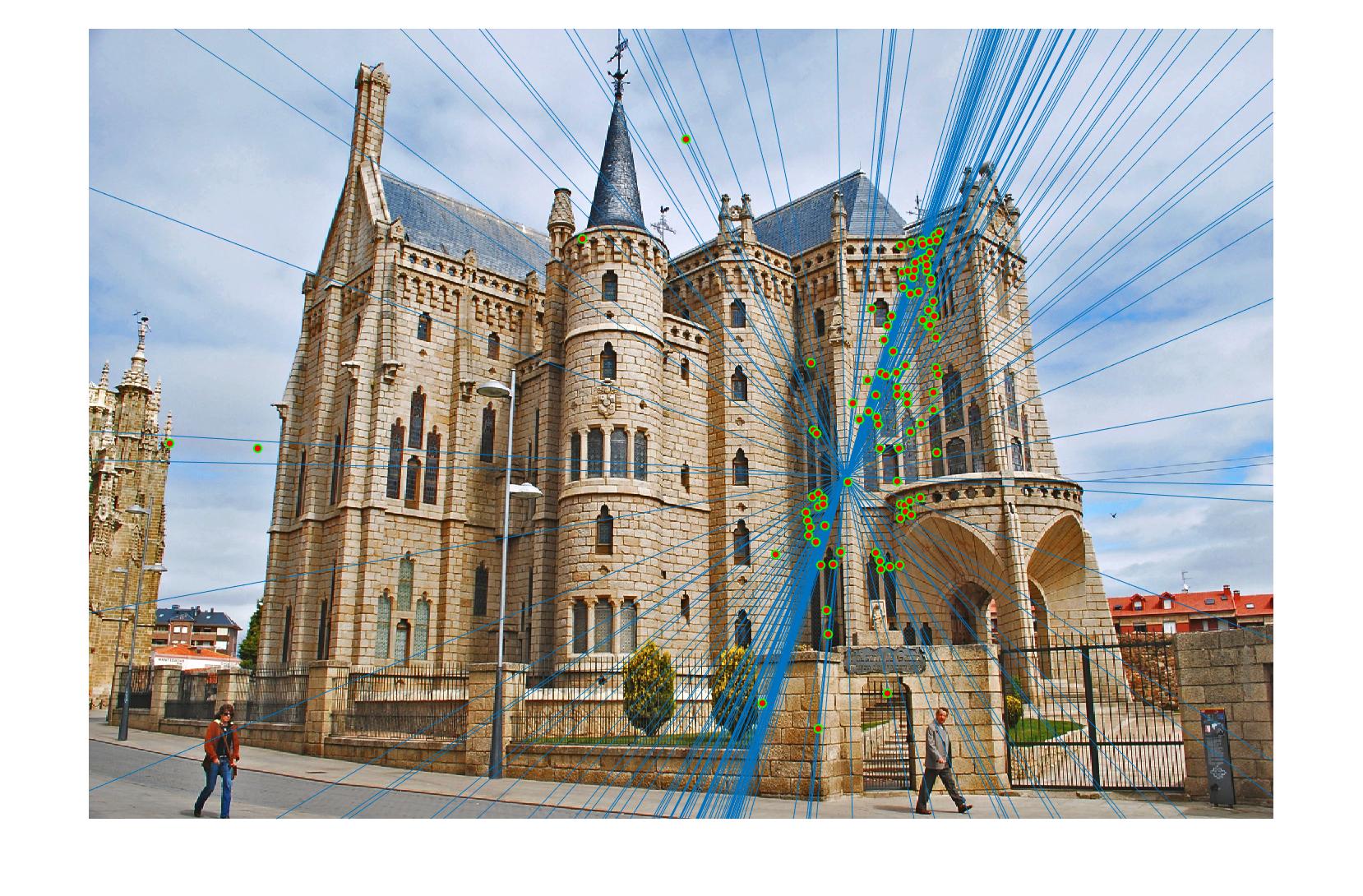
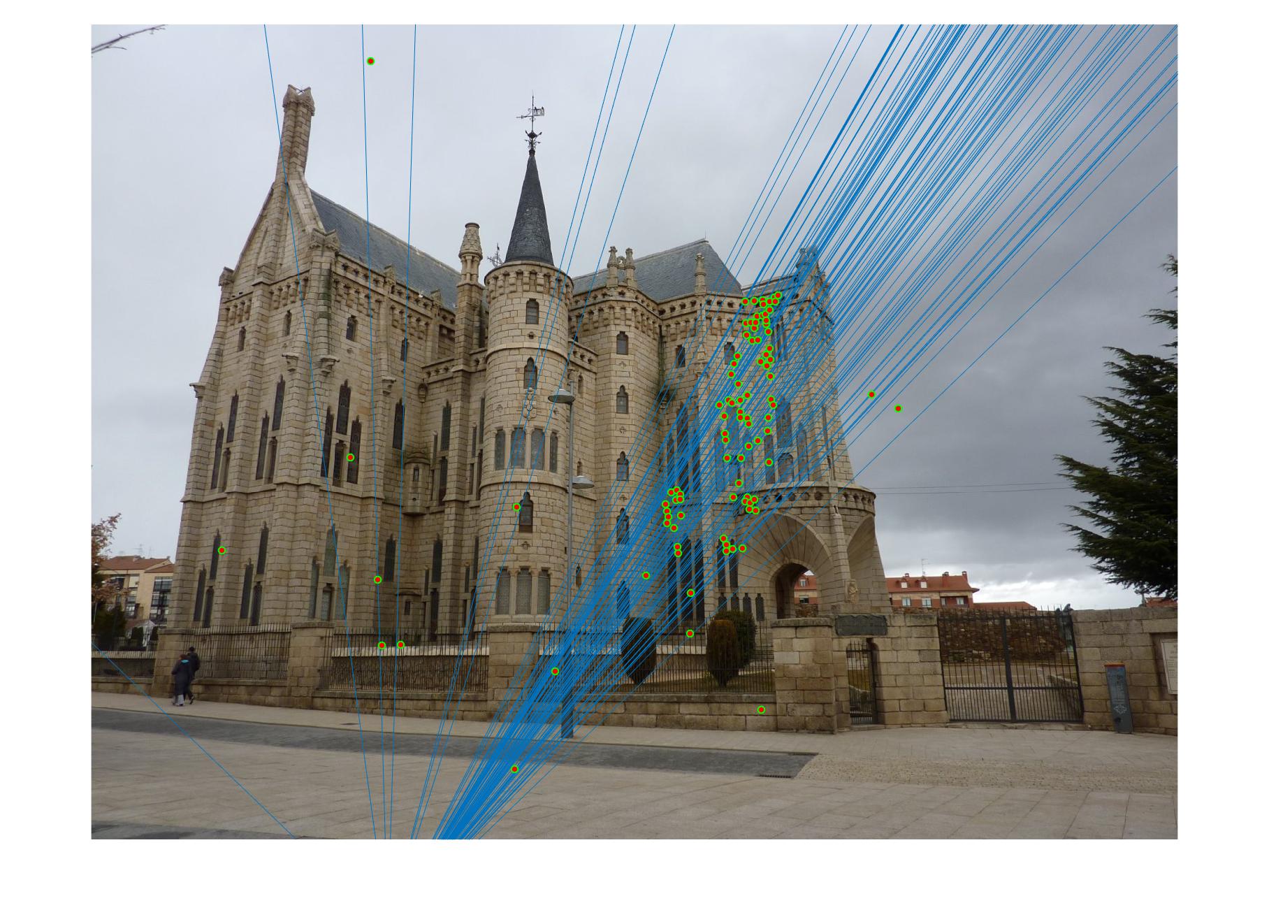
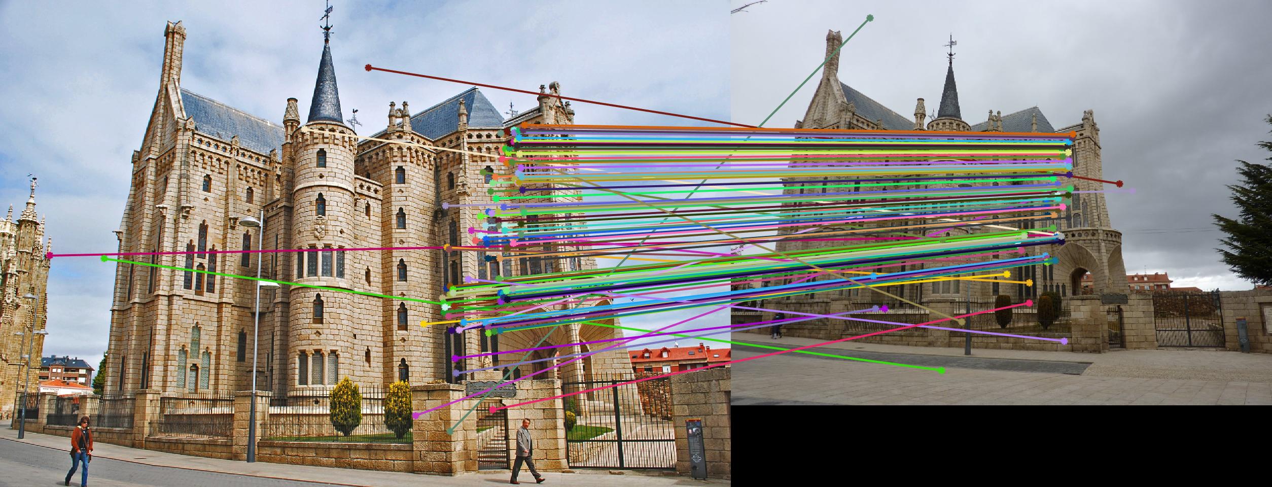
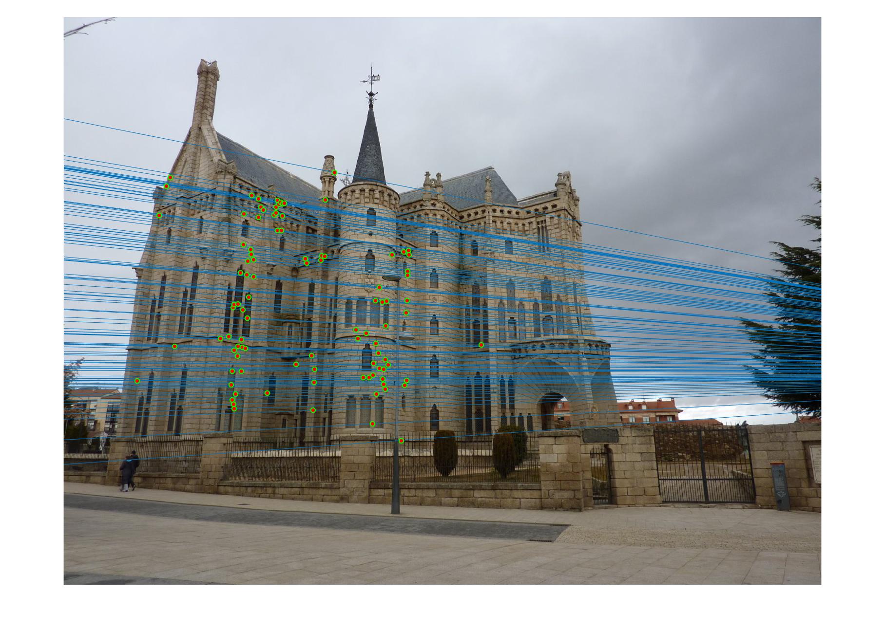
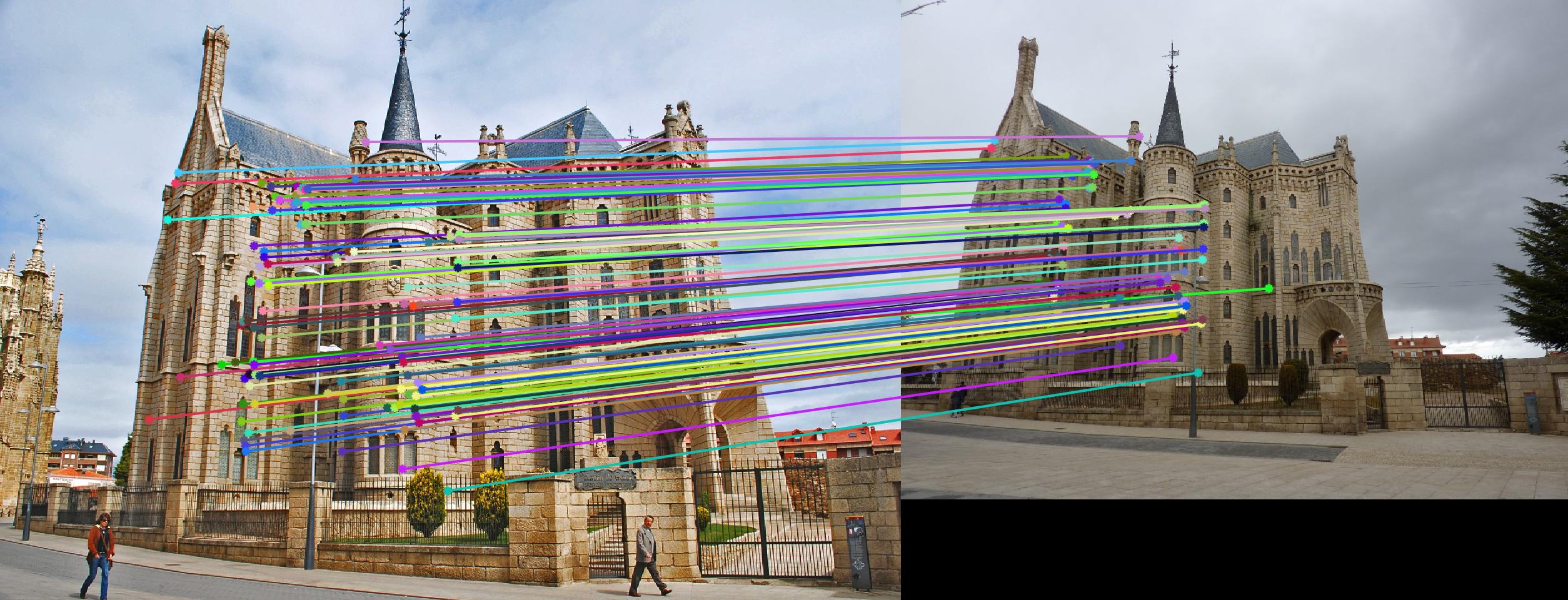
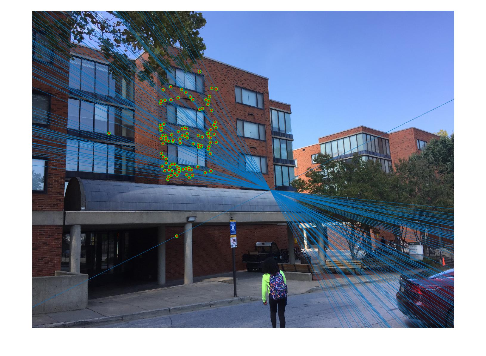
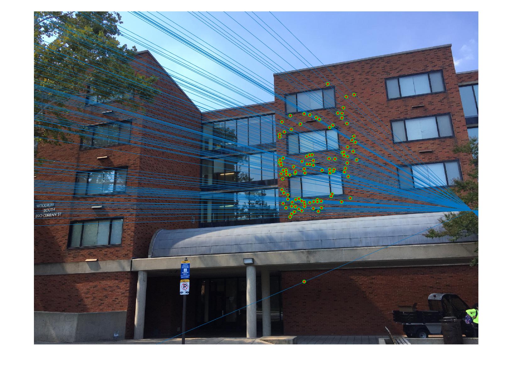
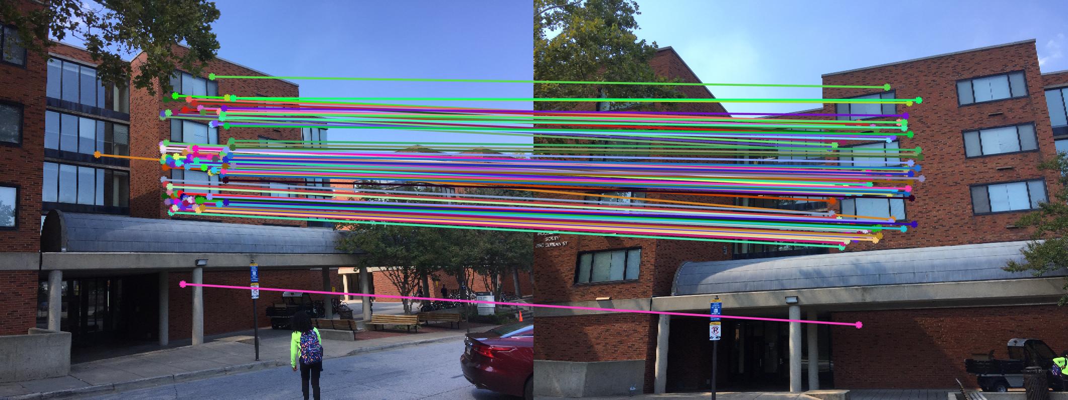
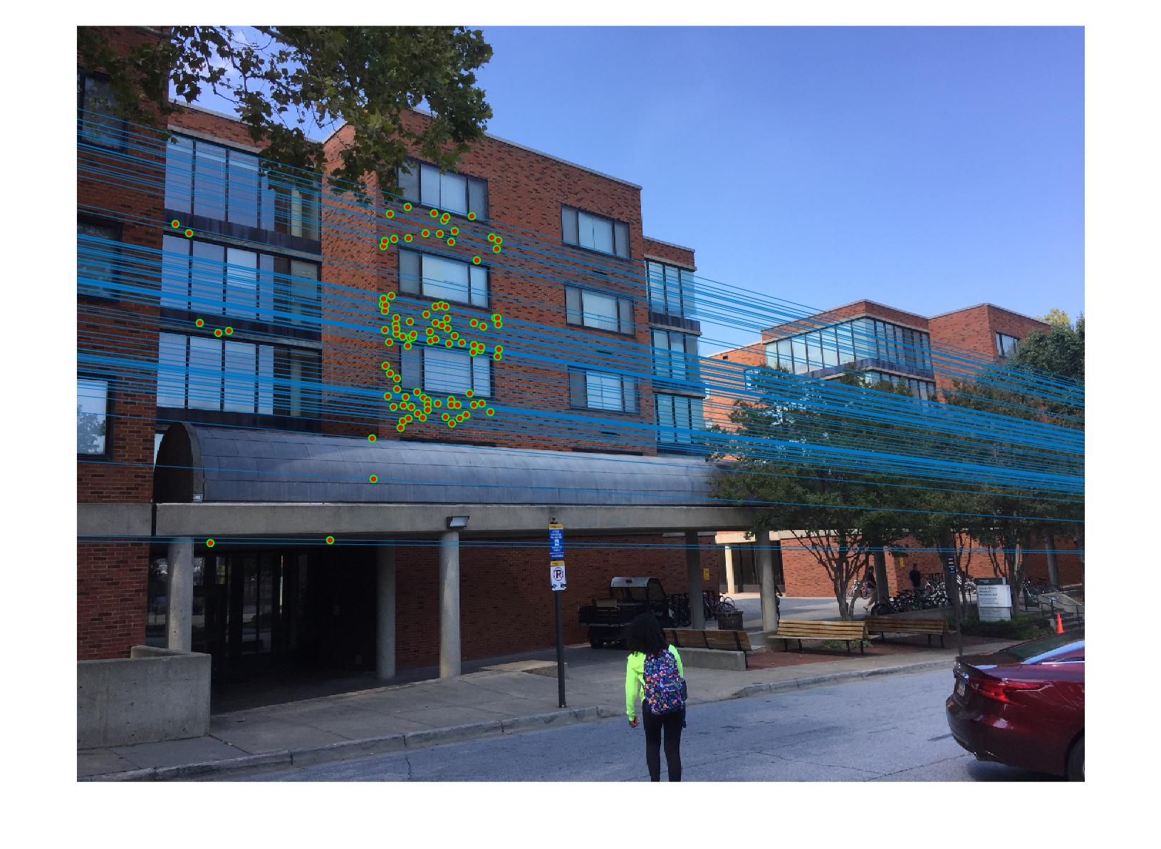
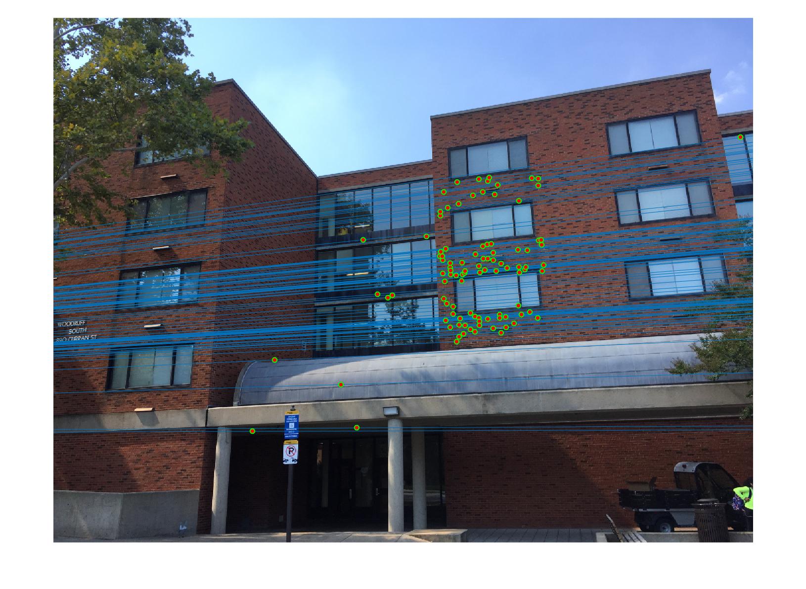
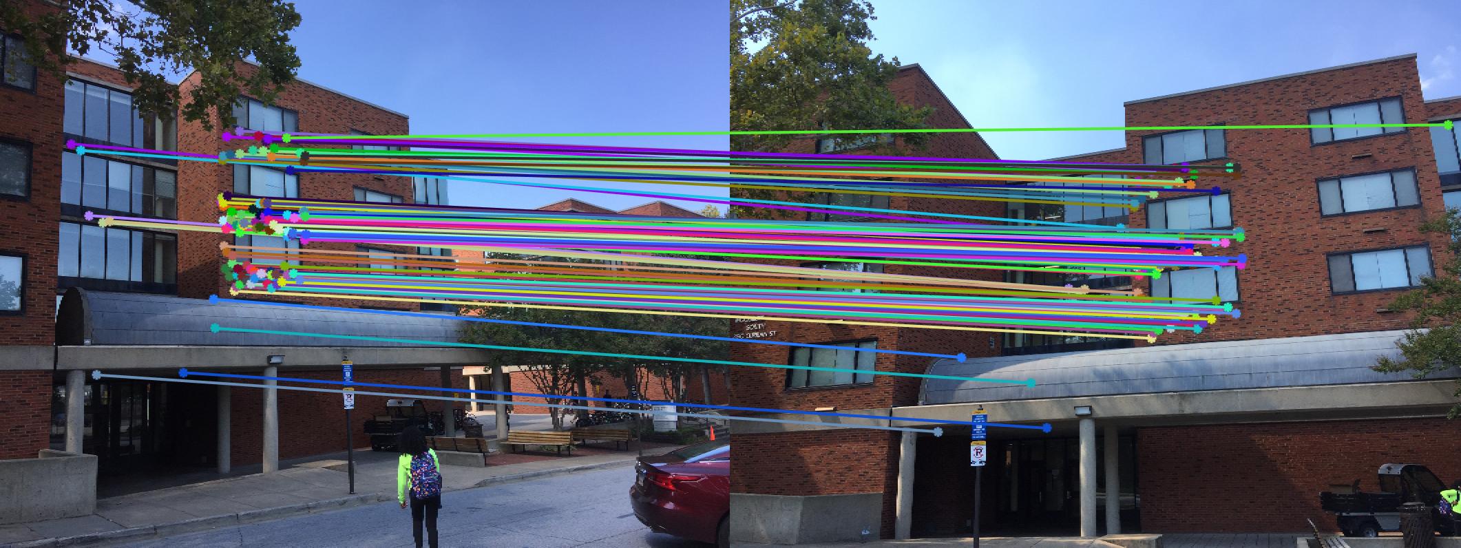
To estimate fundamental matrix with RANSAC, I repeat the following step for 10000 iterations: randomly pick 9 correspondent point pairs and compute the fundamental matrix, and then count the number of inliers(a threshold 0.002 is applied here). The fundamental matrix which yields the maximum number of inliers is eventually returned.

num_samples = 9;
dim = size(matches_a,2);
sample_a = zeros(num_samples,dim);
sample_b = zeros(num_samples,dim);
inliers_a = [];
inliers_b = [];
[row,col] = size(matches_a);
maximum = 0;
% threshold between inliers and outliers
threshold = 0.002;
num_iterations = 10000;
max_inliers = 100;

for ii = 1:num_iterations
    temp_a = [];
    temp_b = [];
    rand_samples = randperm(row,num_samples);
    for i = 1:num_samples
        sample_a(i,:) = matches_a(rand_samples(i),:);
        sample_b(i,:) = matches_b(rand_samples(i),:);
    end
    % calculate fundatmental matrix
    F = estimate_fundamental_matrix(sample_a,sample_b);
    count = 0;
    %ransac
    for i = 1:row
        % count number of  inliers
        if (abs([matches_b(i,:),1]*F*[matches_a(i,:),1]') <= threshold)
            count = count+1;
            temp_a = [temp_a;matches_a(i,:)];
            temp_b = [temp_b;matches_b(i,:)];
        end
    end
    if(count > maximum)
        maximum=count;
        inliers_a = temp_a;
        inliers_b = temp_b;
        Best_Fmatrix = F;
    end 
end
if size(inliers_a,1) > max_inliers
    inliers_a=inliers_a(1:max_inliers,:);
    inliers_b=inliers_b(1:max_inliers,:);
end

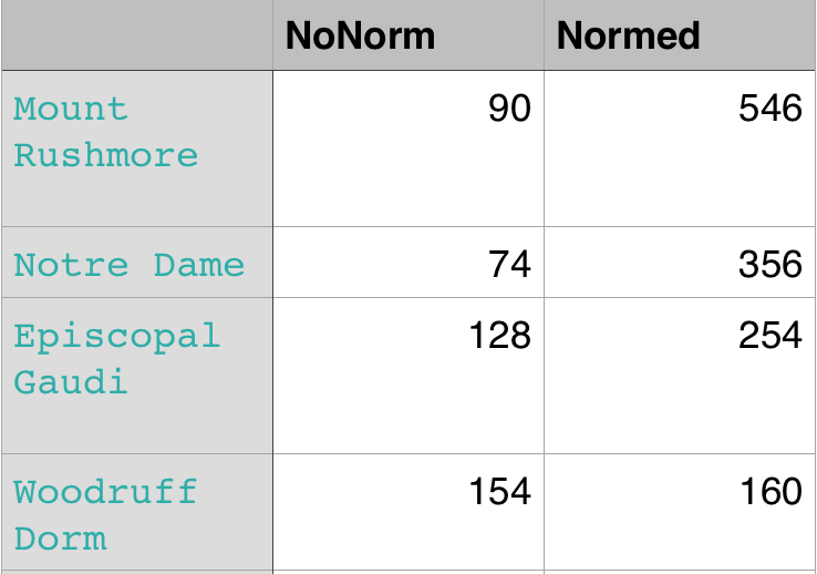
Results in a table