Project 3 Camera Calibration and Fundamental Matrix Estimation with RANSAC
Part I: Camera Projection Matrix
The goal is to compute the projection matrix that goes from world 3D coordinates to 2D image coordinates. Recall that using homogeneous coordinates the equation for moving from 3D world to 2D camera coordinates is:
Another way of writing this equation is:
Thus we get a homogeneous linear system:
In my implementation, I solve this linear least squares problem by SVD:
	[U, S, V] = svd(A);
	M = V(:, end);
	M = reshape(M, [], 3)';
Part I: result
My estimate of the projection matrix is:
My estimate of the camera center is:
Part II: Fundamental Matrix Estimation
The next part of this project is estimating the mapping of points in one image to lines in another by means of the fundamental matrix. This will require you to use similar methods to those in part 1. We will make use of the corresponding point locations listed in pts2d-pic_a.txt and pts2d-pic_b.txt. Recall that the definition of the Fundamental Matrix is:
Which is the same as:
Still I use SVD to solve the regression equations.
To enforce the rank-2 constraint of fundamental matrix, we can also use SVD:
	[U, S, V] = svd(F_matrix);
	S(3,3) = 0;
	F_matrix = U * S * V';
Part II: result
The fundamental matrix for the base image pair I estimate is:
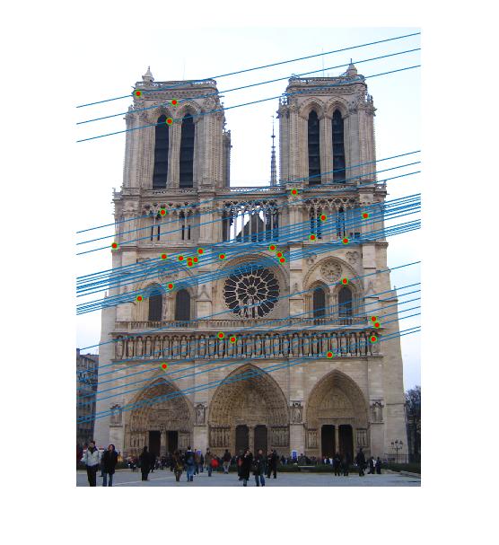
Epipolar lines are shown as:
 |
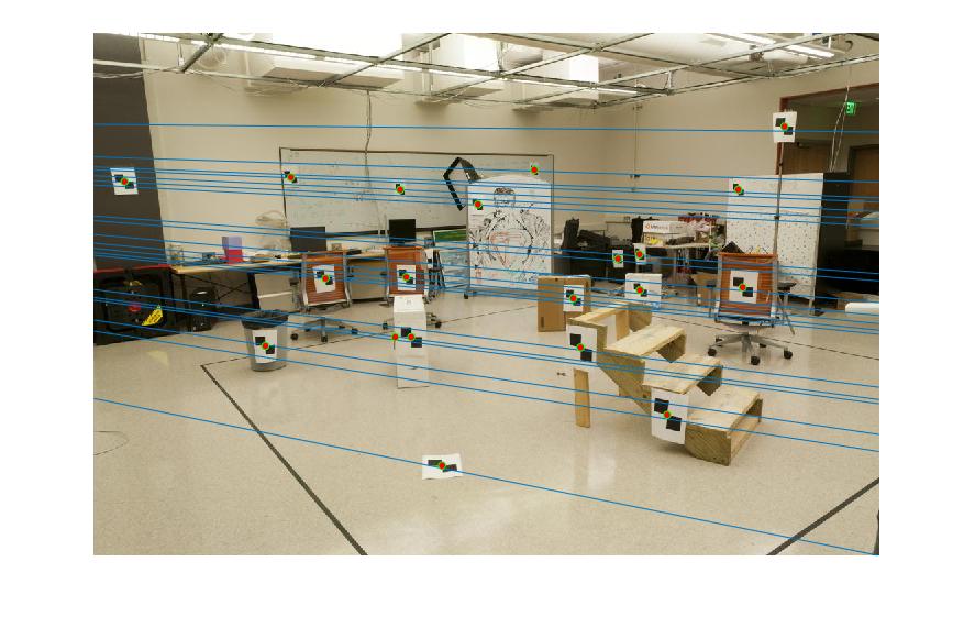 |
Figure 1.Epipolar lines of base image pair
Part III: Fundamental Matrix with RANSAC
We use VLFeat to do SIFT matching. We'll use these putative point correspondences and RANSAC to find the "best" fundamental matrix.
A very important problem is how we define the distance metric for inliers and outliers.
Recall the properties fundamental matrix has, we can define distance as:
So the distances of correct epipolar match correspondences are approximately 0.
As for the number of iterations, I just fix it at 1000. In most cases, it works well in my experiment.
Part III: Result
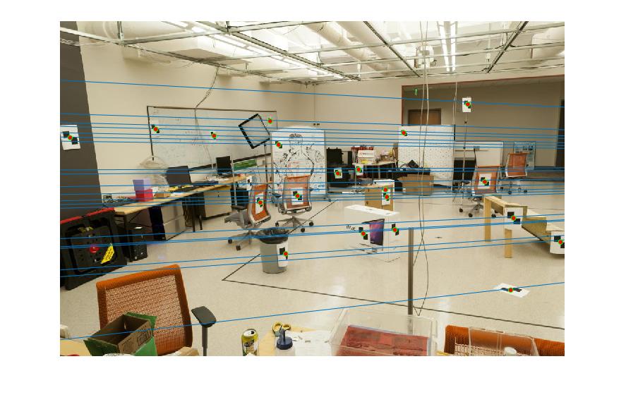
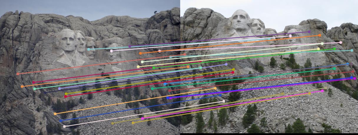
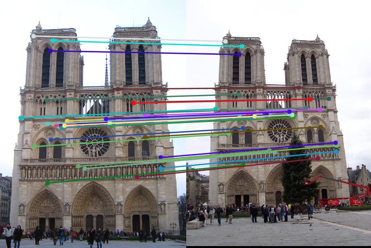
In the experiment, there may be many inliers with the best estimated fundamental matrix. For the visual clarity, I randomly choose 30 of these inliers
 |
 |
 |
|
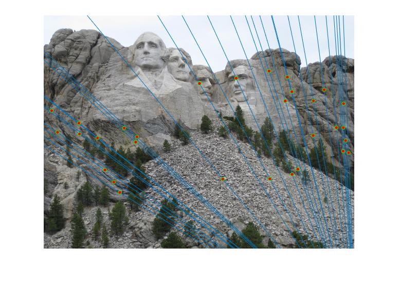
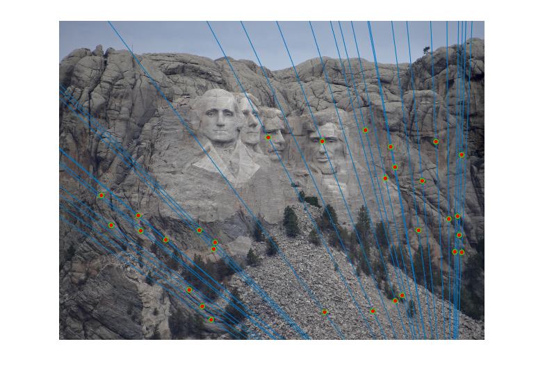
Figure 2.Epipolar lines and correspondance of Mount Rushmore
 |
 |
 |
|
Figure 3.Epipolar lines and correspondance of Notre Dame
Part IV Extra Credit: Normalized coordinates
linear method consists in finding the least eigenvector of the matrix \(A^{T}A\). Acording to work of Richard I. Hartley, the condition number of the matrix \(A^{T}A\) may be very poor so very small changes to the data can cause large changes to the solution.
To make the estimate of fundamental matrix better, we can normalize the coordinates before computing the fundamental matrix. The basic step is
- The points are translated so that their centroid is at the origin.
- The points are then scaled isotropically so that the average distance from the origin is equal to \(\sqrt{2}\)
	nPoints = size(Points, 1);
	Center = sum(Points) / nPoints;
	Translate = [1, 0, 0; 0, 1, 0; -Center(1), -Center(2), 1]';
	Points = Points - ones(nPoints, 1) * Center;
	DistanceSum = sum(sqrt(Points(:, 1) .^ 2 + Points(:, 2) .^ 2));
	Lambda = DistanceSum / nPoints / sqrt(2);
	Scale = [1 / Lambda, 0, 0; 0, 1 / Lambda, 0; 0, 0, 1]';
	transformation = Scale * Translate;
	T_a = compute_transformation_matrix(Points_a);
	T_b = compute_transformation_matrix(Points_b);
	Homo_a = ones(nPoints, 3); Homo_b = ones(nPoints, 3);
	Homo_a(:, 1 : 2) = Points_a; Homo_b(:, 1 : 2) = Points_b;
	Normalized_Homo_a = Homo_a * T_a';
	Normalized_Homo_b = Homo_b * T_b';
F_matrix = T_b' * F_matrix * T_a;
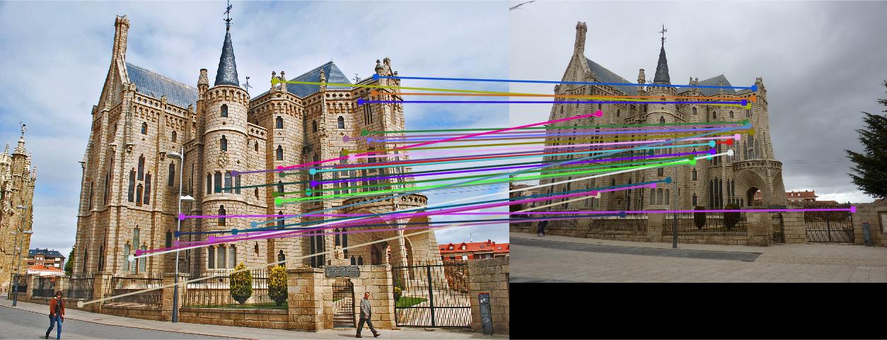
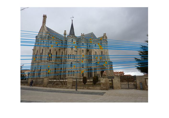
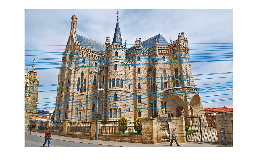
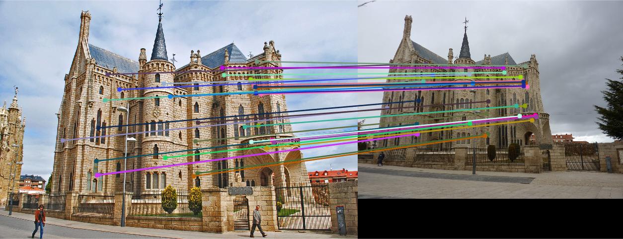
Part IV Extra Credit: Result
 |
 |
 |
|
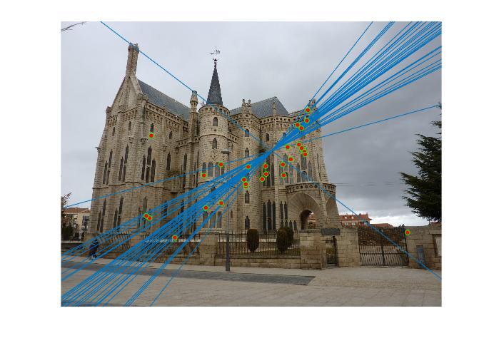
Figure 4.Epipolar lines and correspondance of non-normalized Episcopal Gaudi
 |
 |
 |
|
Figure 5.Epipolar lines and correspondance of normalized Episcopal Gaudi
As we can see, normalized coordinates largely improve the results of Episcopal Gaudi pair. If we don't use normalization, the result seems totally wrong: large error of epipolar lines and wrong correspondence.
References
[1] R Hartley. In Defence of the 8-point Algorithm. IEEE Tr. on PAMI, 1997.