Project 3: Camera Calibration and Fundamental Matrix Estimation with RANSAC
  |
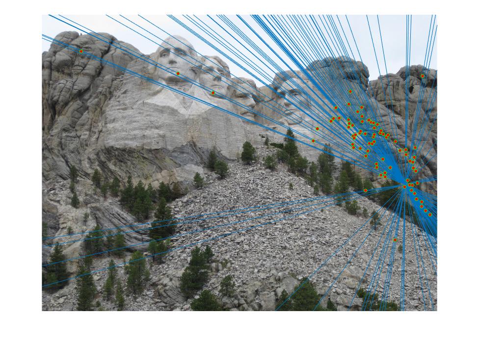
| Multiple Views of Mount Rushmore |
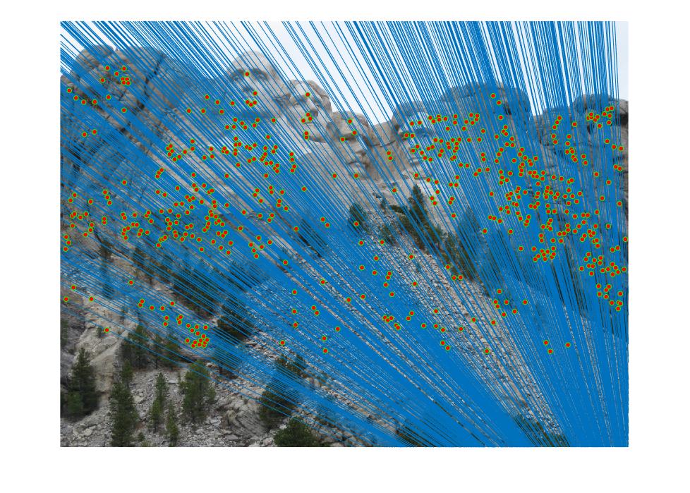
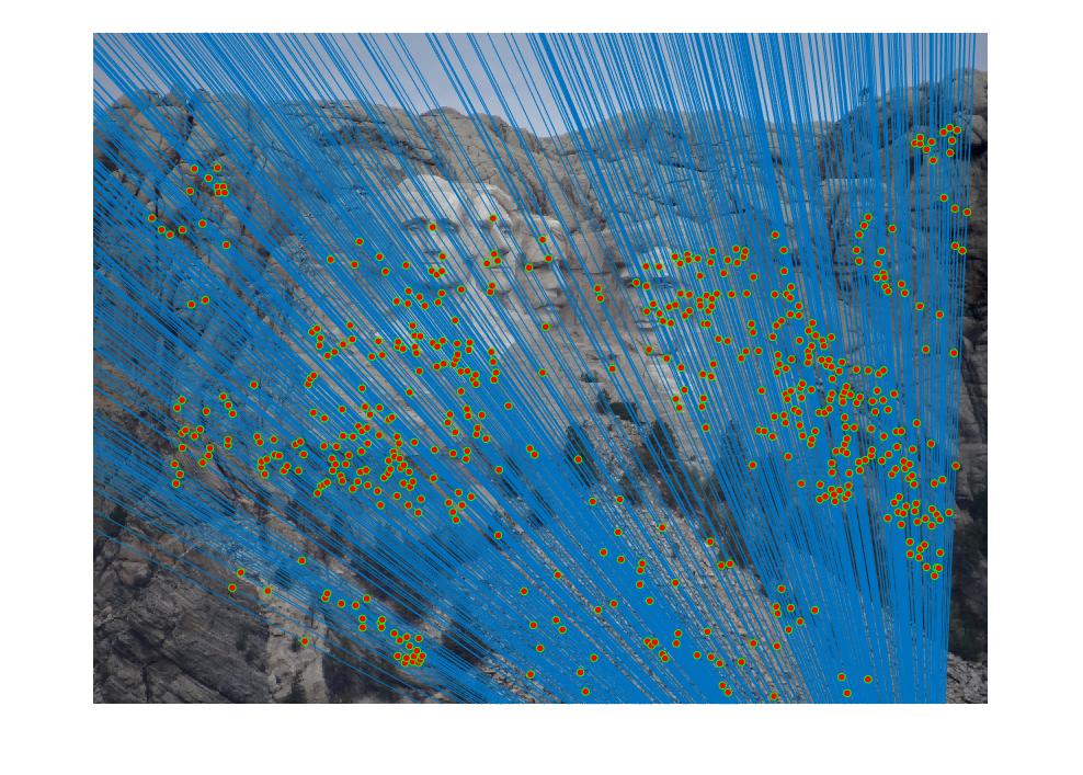
The objective of the project Camera Calibration and Fundamental Matrix Estimation with RANSAC is to estimate the camera projection matrix and the fundamental matrix, in order to visualize matches between two different views of the same scene.
An output of the project is shown above. Two views of Mount Rushmore are presented with epipolar lines and point matches marked. The overall accuracy is close to 100%, which is a lot better than the basic SIFT feature matching algorithm.
Methodology
The program implementation includes Camera Projection Matrix, Fundamental Matrix Estimation and RANSAC. The Methodology section will cover each of them.
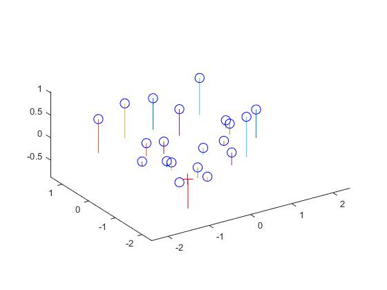
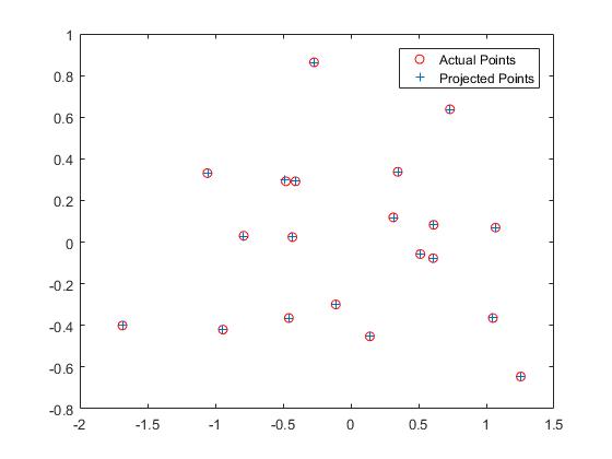
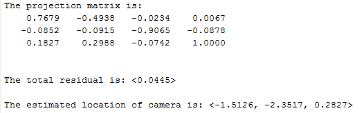
1. Camera Projection Matrix
The projection matrix is calculated by solving the matrix constructed by existing matches of 3D and 2D coordinates. The matrix Ax=b is solved by using the matlab command x = A\b. The residual of the regression is at a low level of 0.0445. Below is a presentation of the results.
 |
 |
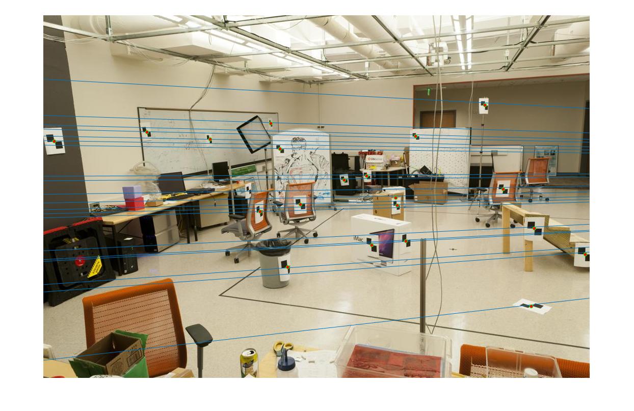
| View of the scene | Projection visualization |
 |
| Part1 Result |
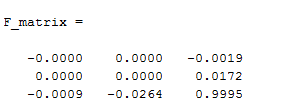
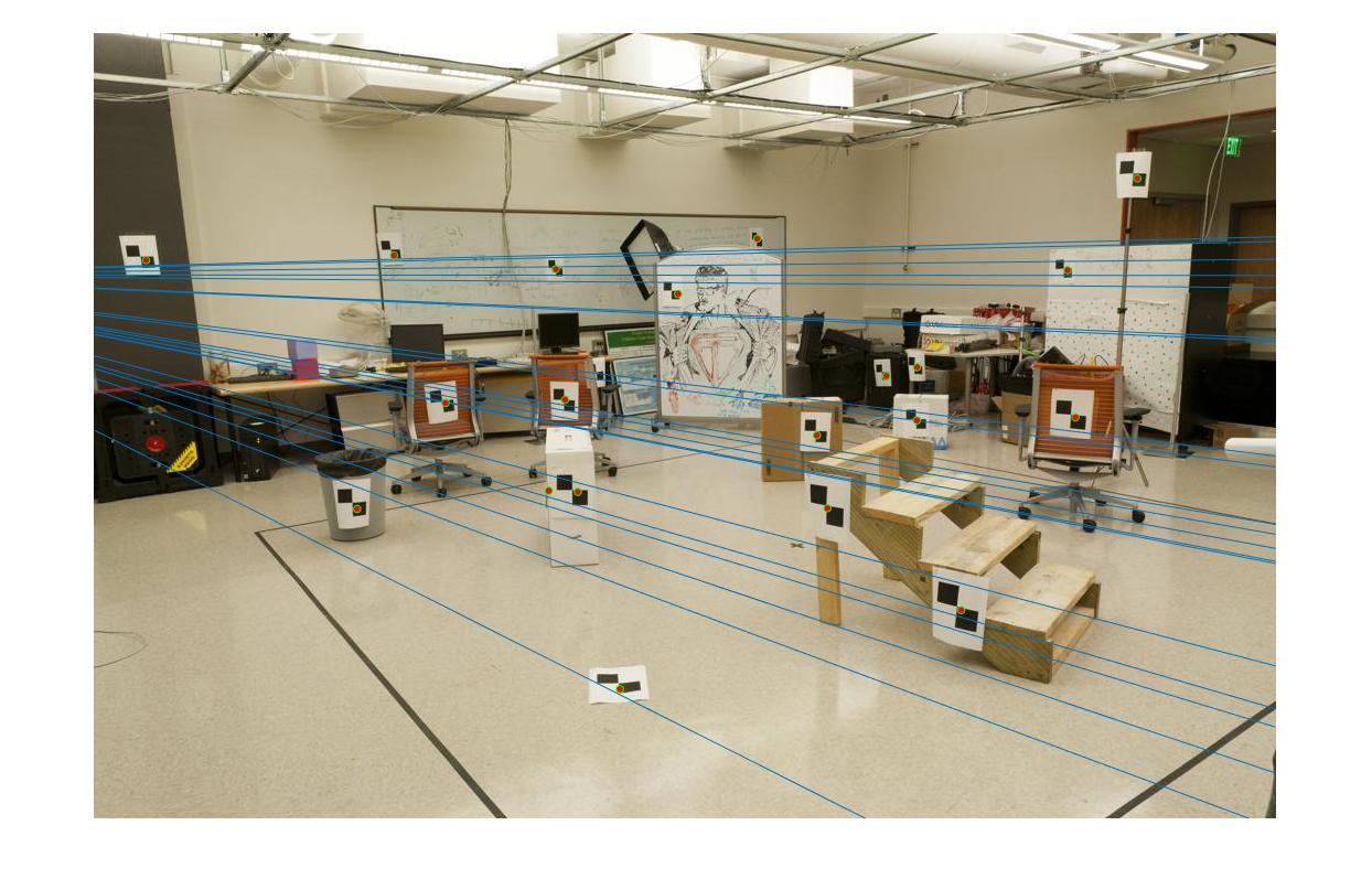
2. Fundamental Matrix Estimation
Similar to part 1, the fundamental matrix is solved by solving the regression problem. However, it is solved with singular value decomposition. Below is the result display.
 |
| View 1 |
 |
| View 2 |
 |
| Part2 Result |
3. Fundamental Matrix with RANSAC
In part 3, the SIFT features are found by the VLFeat package as the input. The program uses RANSAC algorithm to obtain the best-match fundamental matrix. In each iteration, a number of points are randomly chosen for calculating the fundamental matrix. Then the matrix is tested among all the matches in the input. The matrix with the most inliers would be selected.
The number of points for calculating the fundamental matrix is set to 8. The threshold distinguishing between inliers and outliers is set to be 0.003. The algorithm terminates whenever a fundamental matrix matches all the points (which is a rare case) or a maximum number of iterations is reached, which is set to 1000 in my implementation.
The implementation is shown as follows.
% Homegeneous coordinates
one = ones(dataSize, 1);
homo_coor_a = [matches_a one];
homo_coor_b = [matches_b one];

while iteration<=max_iteration
    index = rand(num_of_points, 1);
    index = ceil(index*dataSize);
    points_a = matches_a(index, :);
    points_b = matches_b(index, :);
    currentFmatrix = estimate_fundamental_matrix(points_a, points_b);

    score = dot((homo_coor_b * currentFmatrix)', homo_coor_a')';
    score = abs(score)max_inliers
        Best_Fmatrix = currentFmatrix;
        max_inliers = num_inliers;
        inliers = find(score);
        if max_inliers == dataSize
            break
        end
    end

    iteration = iteration + 1;

end
Two results are shown as follows.
 |
| Mount Rushmore View 1 |
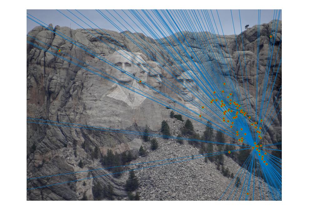 |
| Mount Rushmore View 2 |
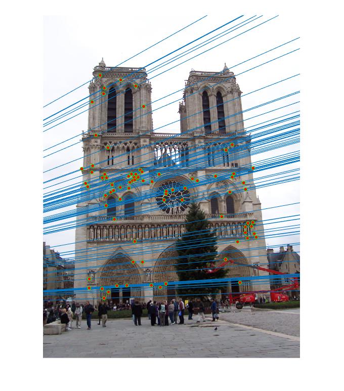 |
| Notre Dame View 1 |
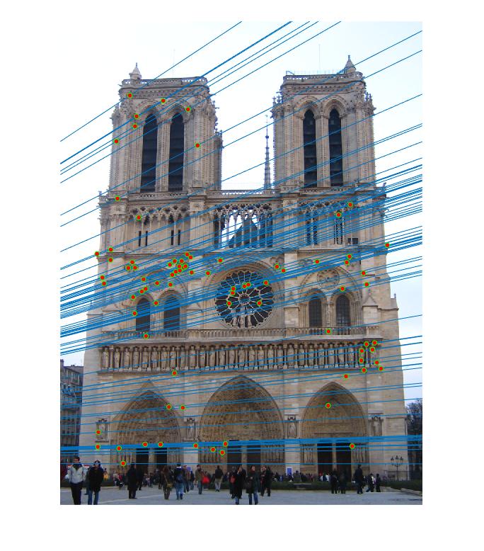 |
| Notre Dame View 2 |
Extra Points Implementation
The normalization of the coordinates is implemented to enhance the performance of the whole system.
| Transformation Equation |
The coordinates are normalized to zero mean and sqrt(2) average distance by introducing the translation and
scaling matrix. The following steps introduces the flow of execution.
1. Convert the coordinates into homogeneous coordinates.
2. Calculate coordinates mean (Cu, Cv)
3. Construct translation matrix T_translation, as the second matrix on the right hand side of the transformation
equation.
4. Transform the points using the translation matrix.
5. Calculate mean distance of the points to the center (0,0) and the scaling factor is calculted as
desired_distance/average_distance;
6. Construct scaling matrix T_scale, as the first matrix on te right hand side of the transformation equation.
7. Transform the points using the scaling matrix.
8. Calculate the fundamental matrix F_norm.
9. Adjust the fundamental matrix by F = Tb' * F_norm * Ta, where Tb = Tb_scale * Tb_translation and
Ta = Ta_scale * Ta_translation.
Below is my implementation of the normalization.
% Homegeneous coordinates
one = ones(pointSize, 1);
Points_a = [Points_a one];

% Matrix initialization
Ta_translate = eye(3);
Ta_scale = eye(3);
Ta = zeros(3,3);

% Translation matrix
mean_a = mean(Points_a);
Ta_translate(1,3) = -mean_a(1);
Ta_translate(2,3) = -mean_a(2);

% Translate the points
Points_a = (Ta_translate * Points_a')';

% Scaling matrix
distance_a = sqrt(Points_a(:, 1).^2 + Points_a(:, 2).^2);
scale_a = sqrt(2)/mean(distance_a);
Ta_scale(1,1) = scale_a;
Ta_scale(2,2) = scale_a;

% Scale the points
Points_a = (Ta_scale * Points_a')';

% Do the same thing to point set b
...
% Calculate the fundamental matrix
...

% Adjust the fundamental matrix
Ta = Ta_scale * Ta_translate;
F_matrix = Tb' * F_matrix * Ta;
In part 2, the normalization does not improve the performance a lot if the data does not contain noise. With noise, normalization can help a lot in the accuracy, as illustrated by the following images.
 |
| View 1 (Without normalization) |
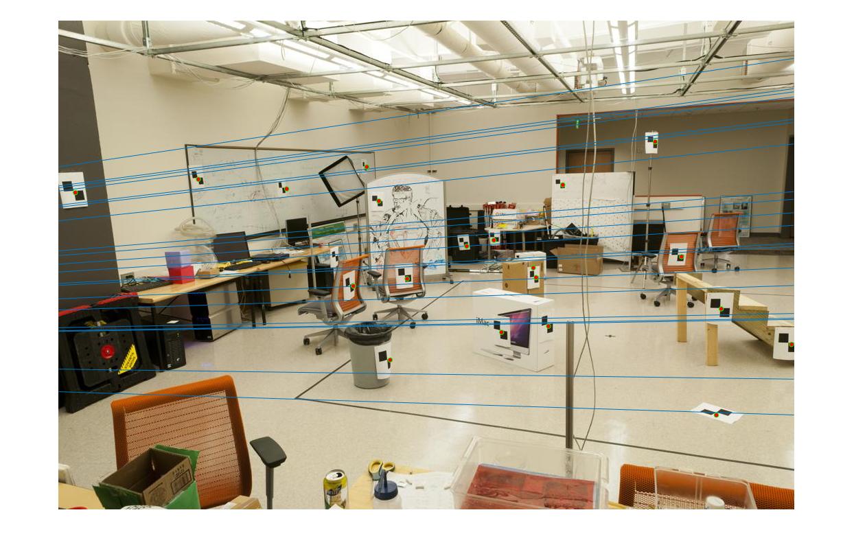 |
| View 2 (Without normalization) |
 |
| View 1 (With normalization) |
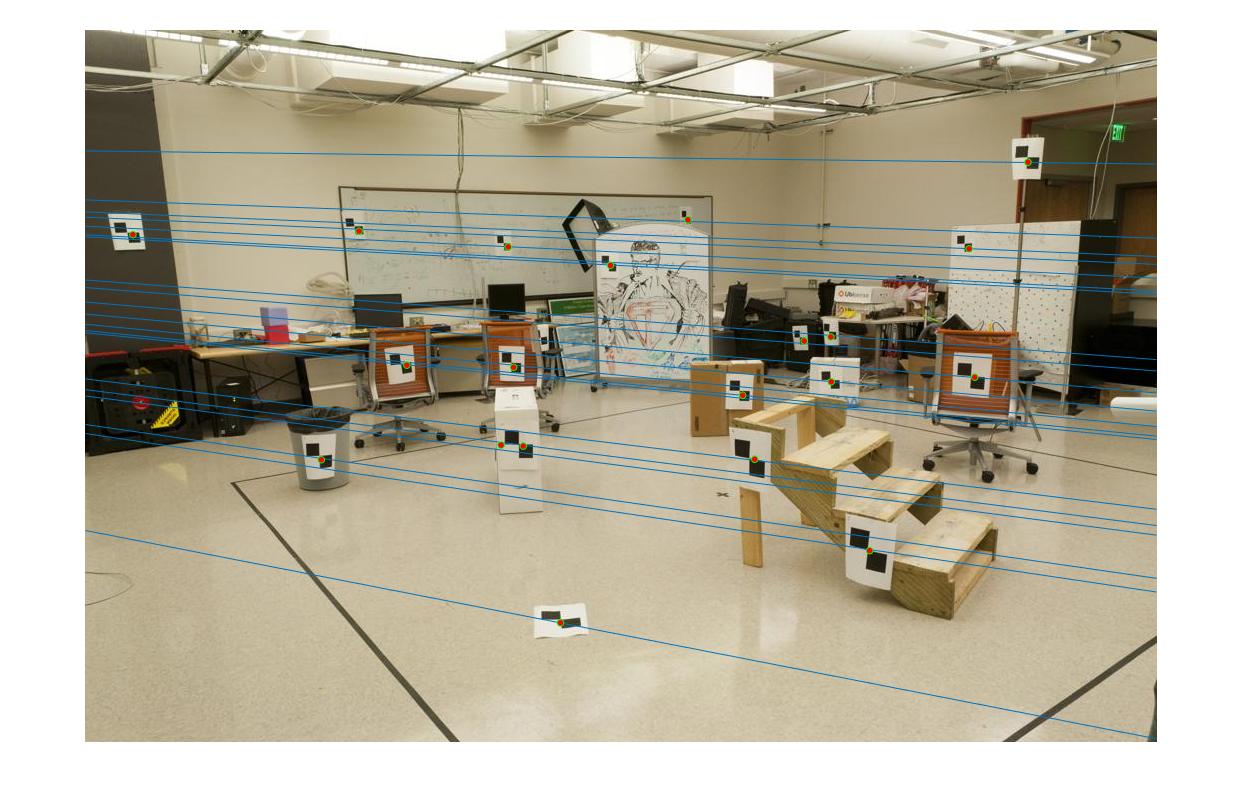 |
| View 2 (With normalization) |
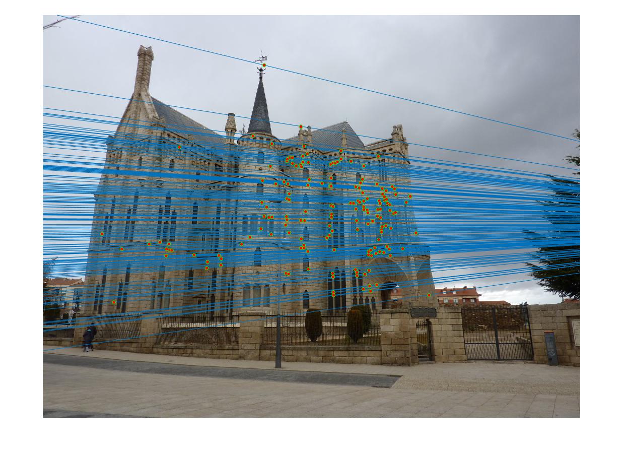
In part 3, the normalization improves the accuracy by a lot, especially for the difficult pairs of images, such as Gaudi. The result is presented as follows. Without normalization the result is still decent in the center but contains a lot of visible errors in the region outside the building. The method with normalization seems to contain no error, except for the match in left bottom corner in image 1. The total number of matches found is 170, with almost no error matches discovered.
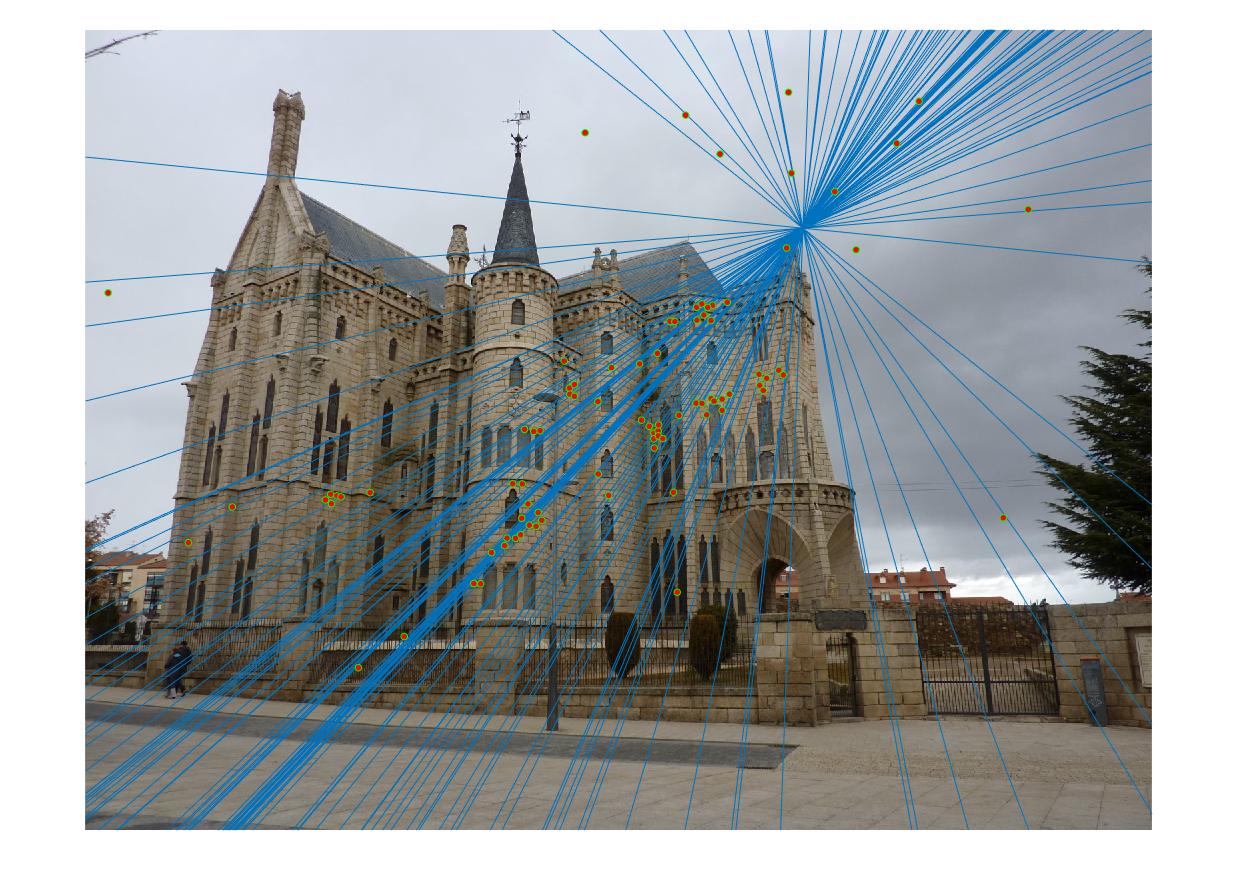 |
| View 1 (Without normalization) |
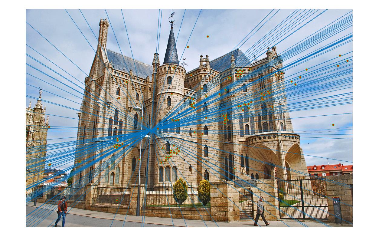 |
| View 2 (Without normalization) |
 |
| View 1 (With normalization) |
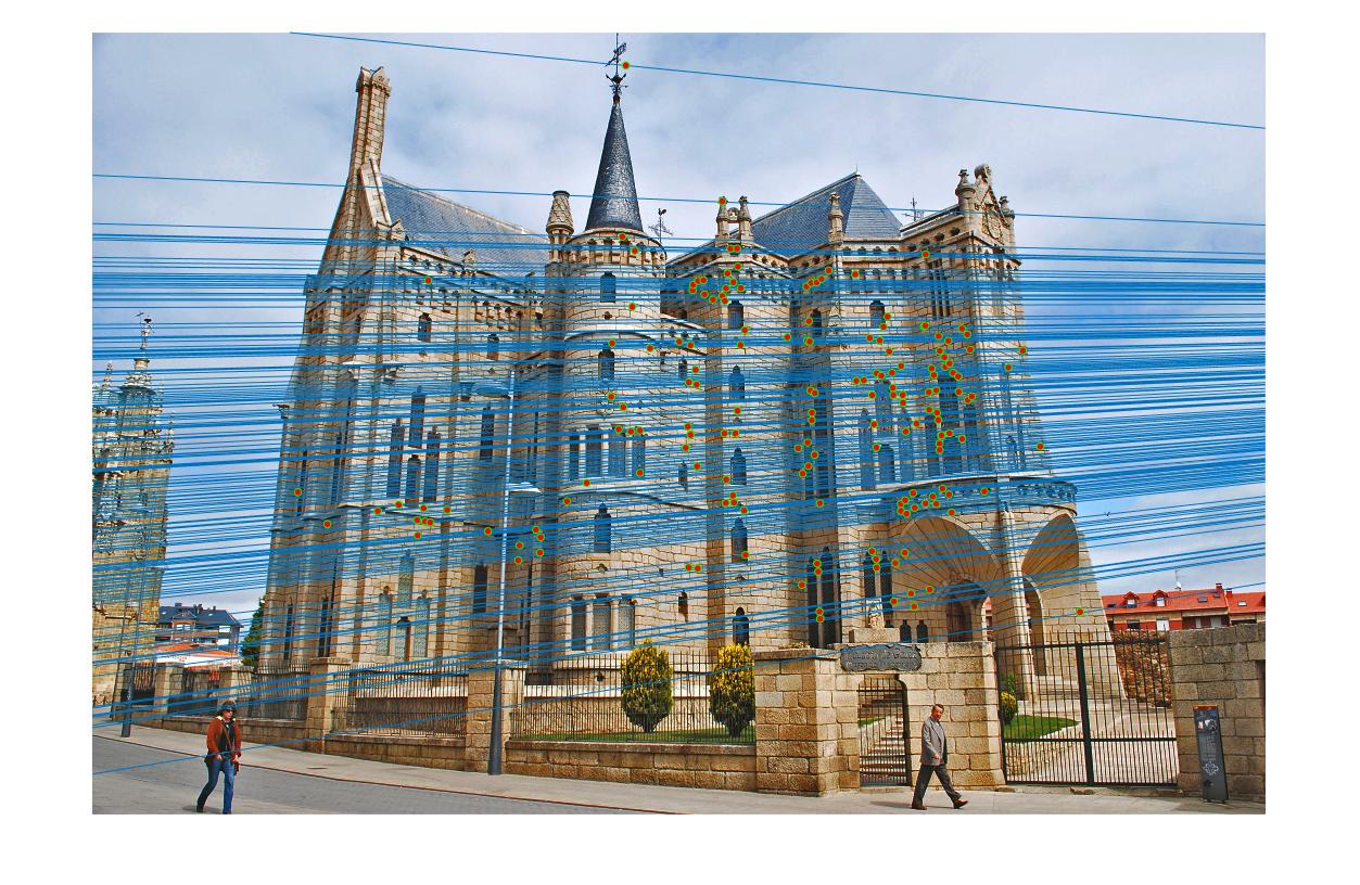 |
| View 2 (With normalization) |
Here is another set of example. The results are already presented in part 3 and here it is used to show that the method with normalization definitely outperforms the one without it.
|
| View 1 (Without normalization) |
|
| View 2 (Without normalization) |
|
| View 1 (With normalization) |
|
| View 2 (With normalization) |