Project 3 / Camera Calibration and Fundamental Matrix Estimation with RANSAC
In this project, I implemented the following:
- Camera Projection Matrix + Camera Position
- Fundamental Matrix Estimation
- Fundamental Matrix with RANSAC
- (Extra Credit) Normalized Coordinates
Camera Projection Matrix + Camera Position
The projection from a 3D point to a 2D point is represented by:
$$ \begin{pmatrix}u \\ v \\ 1\end{pmatrix} \cong \begin{pmatrix}u*s \\ v*s \\ s \end{pmatrix} = M \begin{pmatrix}X \\ Y \\ Z \\ 1 \end{pmatrix} =\begin{pmatrix}m_{11} & m_{12} & m_{13} & m_{14} \\ m_{21} & m_{22} & m_{23} & m_{24} \\ m_{31} & m_{32} & m_{33} & m_{34} \end{pmatrix} \begin{pmatrix}X \\ Y \\ Z \\ 1 \end{pmatrix} $$,where M is the projection matrix from 3D homogeneous coordinate to 2D homogeneous coordinate.
If we have N such pairs, we can have a group of equations. Notice that we still have one degree of freedom. Let's fixed m34 to be 1 and use the original 3D and 2D points (without any scaling). Write them in matrix form:
$$ \begin{pmatrix} X1 & Y1 & Z1 & 1 & 0 & 0 & 0 & 0 & -u1*X1 & -u1*Y1 & -u1*Z1 \\ 0 & 0 & 0 & 0 & X1 & Y1 & Z1 & 1 & -v1*X1 & -v1*Y1 & -v1*Z1 \\ . & . & . & . & . & . & . & . & . & . & . \\ Xn & Yn & Zn & 1 & 0 & 0 & 0 & 0 & -un*Xn & -un*Yn & -un*Zn \\ 0 & 0 & 0 & 0 & Xn & Yn & Zn & 1 & -vn*Zn & -vn*Yn & -vn*Zn \end{pmatrix} \begin{pmatrix} m_{11} \\ m_{12} \\ m_{13} \\ m_{14} \\ m_{21} \\ m_{22} \\ m_{23} \\ m_{24} \\ m_{31} \\ m_{32} \\ m_{33} \end{pmatrix} = \begin{pmatrix} u_1 \\ v_1 \\ . \\ . \\ . \\ . \\ . \\ . \\ . \\ u_n \\ v_n \end{pmatrix} $$Solve this equation gives us the values of matrix M. The code is shown below:
A = [];
b = [];
for i=1:size(Points_2D, 1)
	A = [A; ...
	Points_3D(i,:), 1, zeros(1,4), -Points_2D(i,1)*Points_3D(i,:); ...
	 zeros(1,4), Points_3D(i,:), 1, -Points_2D(i,2)*[Points_3D(i,:)]...
	 ];


	b = [b;Points_2D(i,1);Points_2D(i,2)];
end

m = [A \ b;1];
M = reshape(m, 4,3)';
The following code computes the camera position
Center = - (inv(M(1:3,1:3)) * M(1:3, 4))';
Fundamental Matrix Estimation
Ideally, if a pair of two points (p,q) match, we shall have
$$ q^T F p = 0$$,where F is the fundemental matrix (3 x 3) and p, q are in homogeneous coordinates (p in image A and q in image B).
Given n pairs, we can rewrite:
$$ Ax = \begin{pmatrix} p_{11} q_{11} & p_{12} q_{11} & q_{11} & p_{11} q_{12} & p_{11} q_{12} & q_{12} & p_{11} & p_{12} & 1\\ . & . & . & . & . & . & . & . & .\\ p_{n1} q_{n1} & p_{n2} q_{n1} & q_{n1} & p_{n1} q_{n2} & p_{n1} q_{n2} & q_{n2} & p_{n1} & p_{n2} & 1 \end{pmatrix} \begin{pmatrix} f_{11} \\ f_{12} \\ f_{13} \\ f_{21} \\ f_{22} \\ f_{23} \\ f_{31} \\ f_{32} \\ f_{33} \end{pmatrix} = 0 $$,where p_nk means the k-th coordinate of n-th point in image A.
In general, we don't have perfect matches. Also, when n > 8, we usually have null(A) = {0}. Instead of calculating the null space, we compute SVD of A:
$$ A = USV^T$$Then we just take the vector in V associated with the smallest sigular value to be our solution for x (i.e. F matrix). To ensure rank-2 condition, we perform SVD for F matrix, set the smallest sigular value of F to 0 and recompute the F matrix using the updated sigular values. (Thus we won't have much the error in this process).
The code is shown below.
n = size(Points_a,1);
assert(n>=8);

A = zeros(n,9);
for i=1:n
	u = Points_a(i,:);
	v = Points_b(i,:);
	A(i,:) = [u(1)*v(1), u(2)*v(1), v(1), u(1)*v(2), u(2)*v(2), v(2), u(1), u(2), 1];
end

%%%
[U,S,V] = svd(A);
f_values = V(:,end);
% f_values = f_values / norm(f_values);
%%%


F_matrix = reshape(f_values,3,3)';
[U,S,V] = svd(F_matrix);
F_matrix = U(:,1:2)*S(1:2,1:3)*V';
Fundamental Matrix with RANSAC
I wrote the RANSAC part to perform the following steps:
- Randomly choose 8 matches. Calculate the fundemental matrix using these 8 matches.
- Use the obtain fundemental matrix to calculate yFx for each pair of datapoints (x,y). If error is smaller than some threshold epsilon, add this pair to the inlier pair set.
- If size of the inlier set is larger then one for the best fundemental matrix so far, set this current matrix to be the best matrix and the best count of inliers be the current number.
- Repeat for N times.
By trail and error, I set N = 1000 and epsilon = 1e-2.
(Extra Credit) Normalized Coordinates
I normalized the coordinates by the following precodure:
- Take the detected feature points (from VLFeat) in both image A and image B. Denote them X_A and X_B. X_A should be of size n_A x 3 if using homogenous coord.
- Calculate the pooled mean value of X_A and X_B, then substract both X_A and X_B (so that we have the same amount of shift in data points from both image)
- Calculate the standard derivation of X_A in all 3 dimensions and take the mean of them. Denote this mean as m_A. Normalize X_A using scale 1/m_A. Repeat the same step for X_B.
Results
The projection matrix
The projection matrix is:
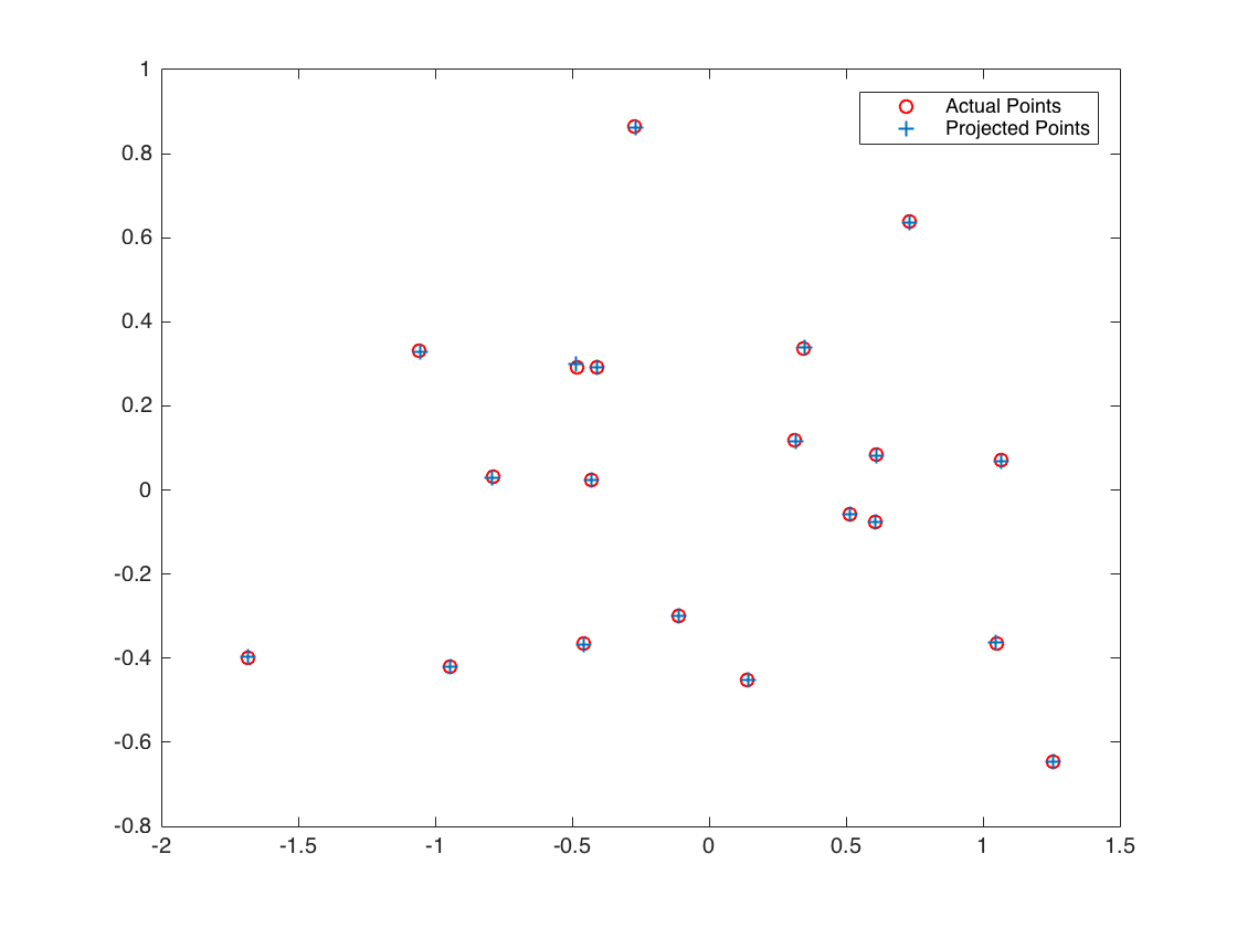
$$ \begin{pmatrix} 0.7679 & -0.4938 & -0.0234 & 0.0067 \\ -0.0852 & -0.0915 & -0.9065 & -0.0878 \\ 0.1827 & 0.2988 & -0.0742 & 1.0000 \end{pmatrix} $$The total residual is: 0.0445
The estimated location of camera is: -1.5126, -2.3517, 0.2827
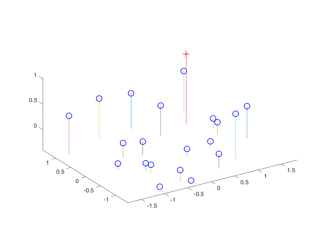
The figures for the estimated projection matrix of the simple example.
Calculation of fundemental matrix
The figures for the estimated fundemental matrix of the simple example, using all 20 pairs of points.
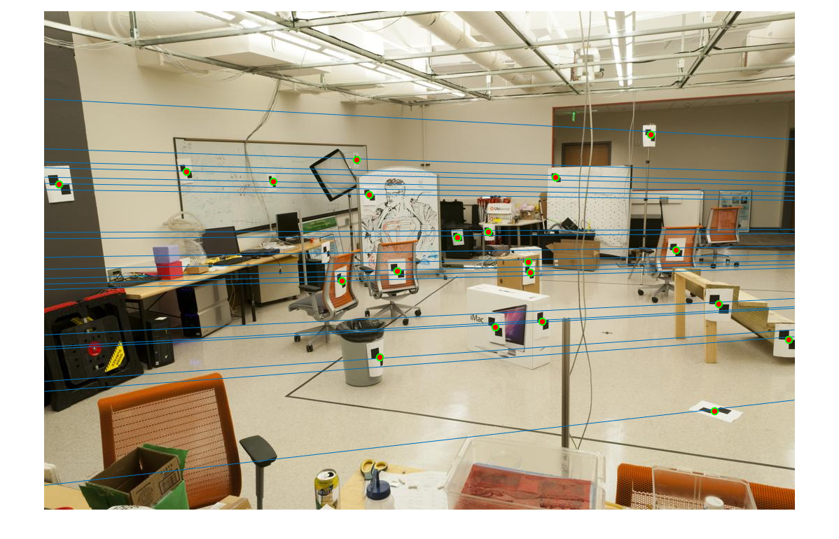
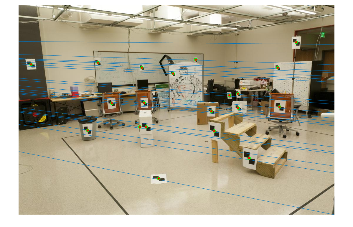
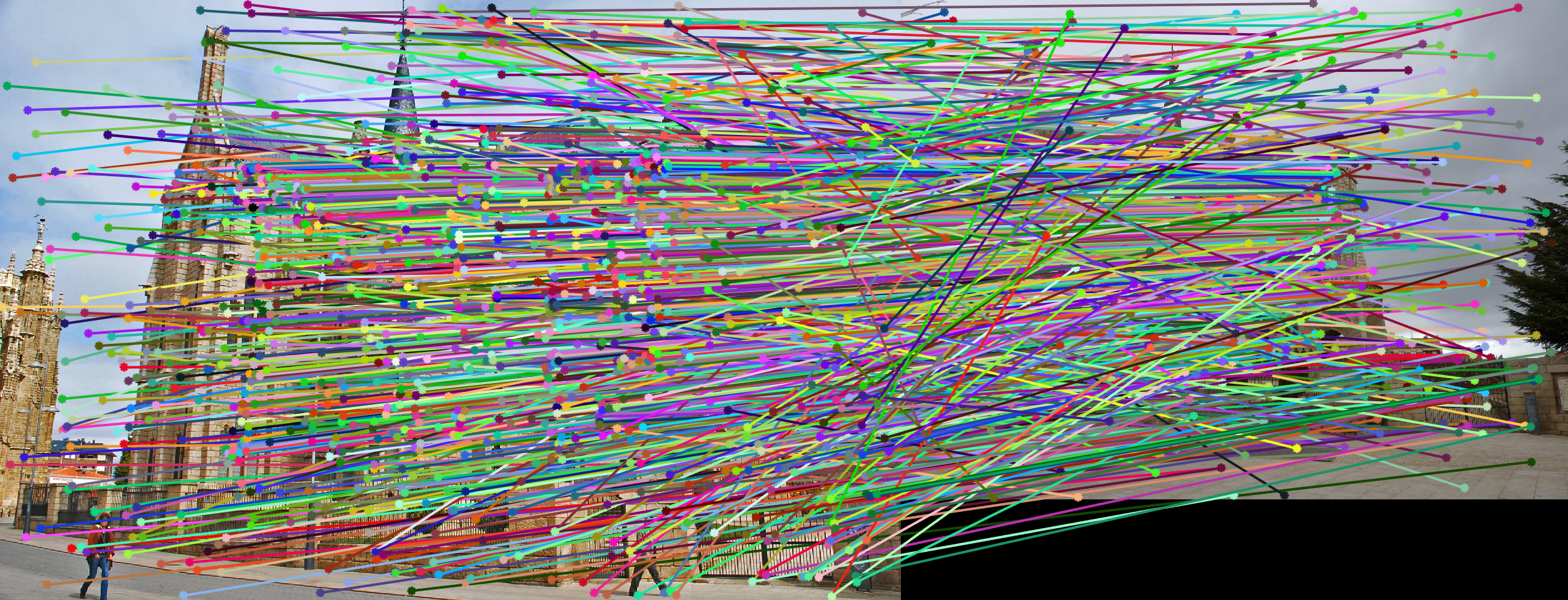
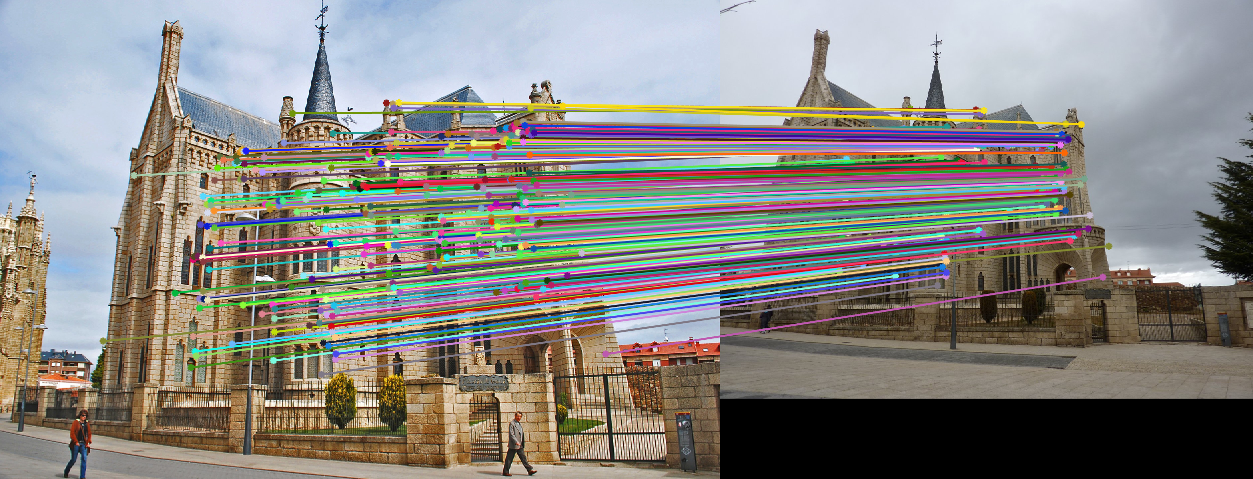
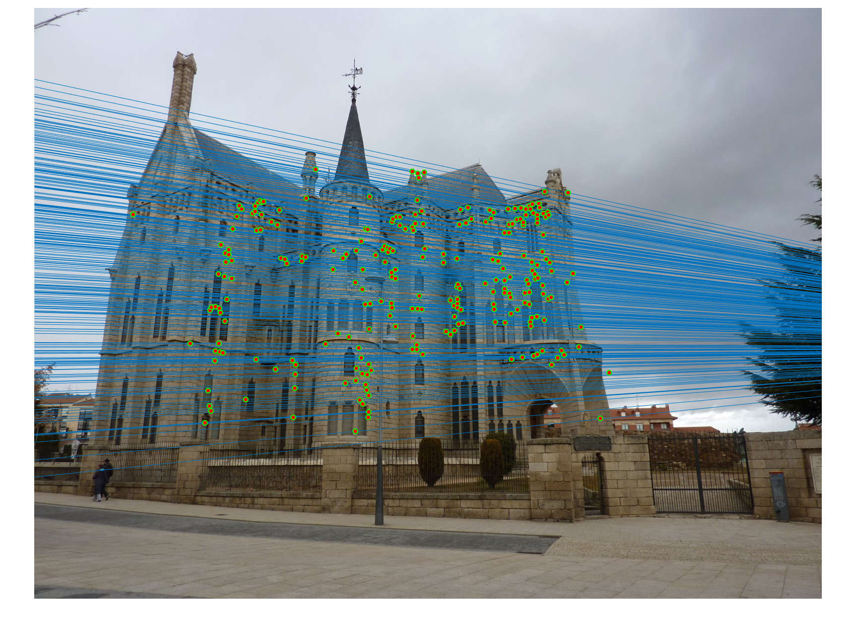
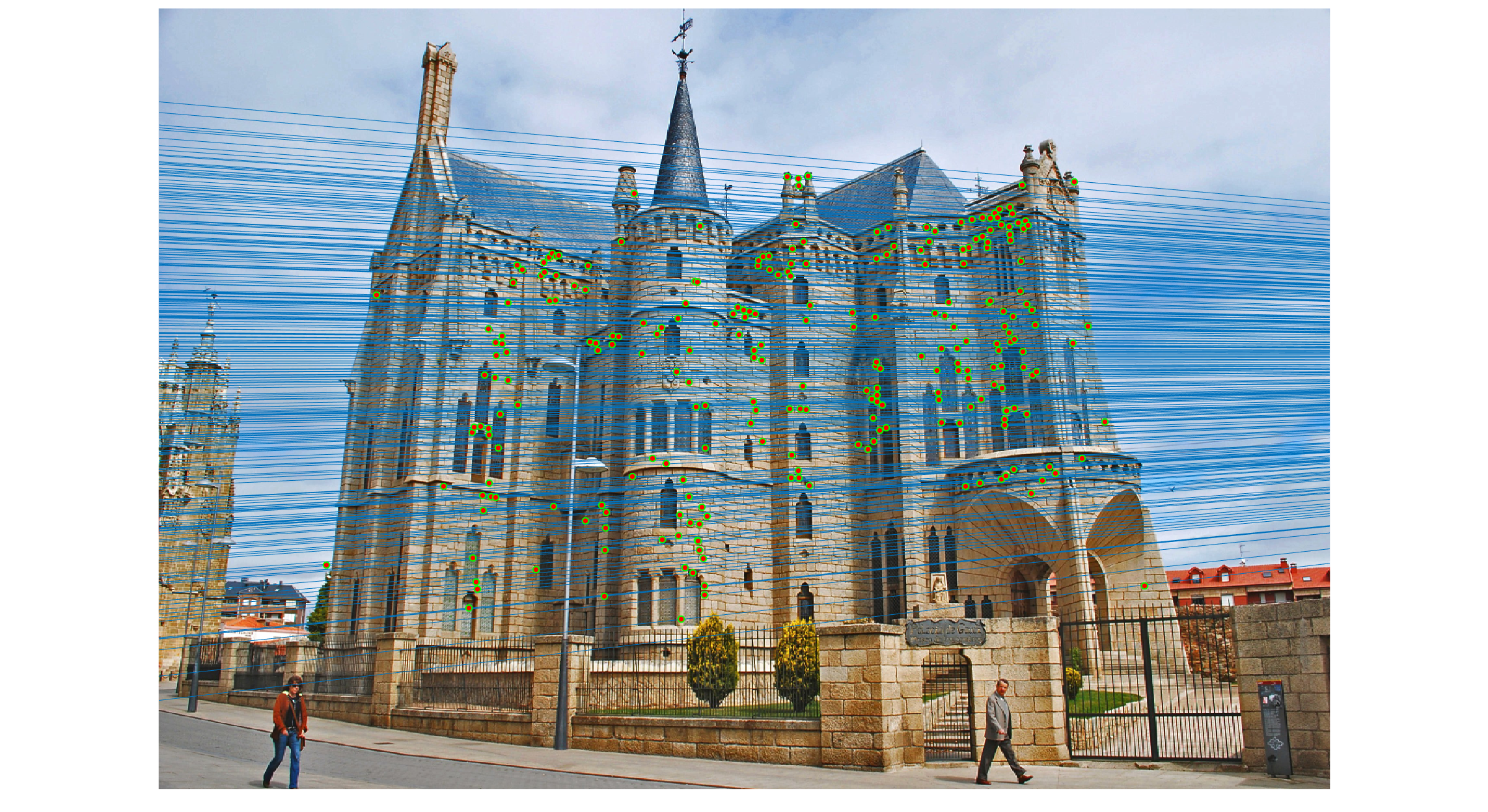
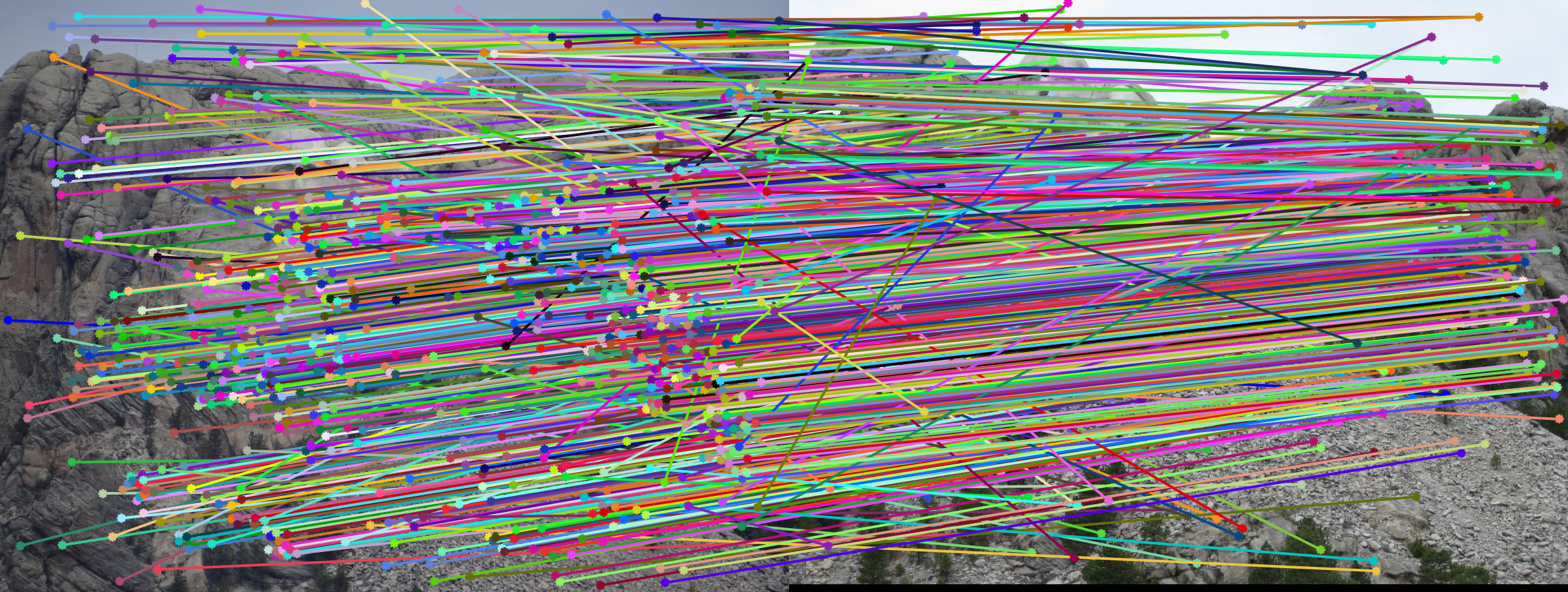
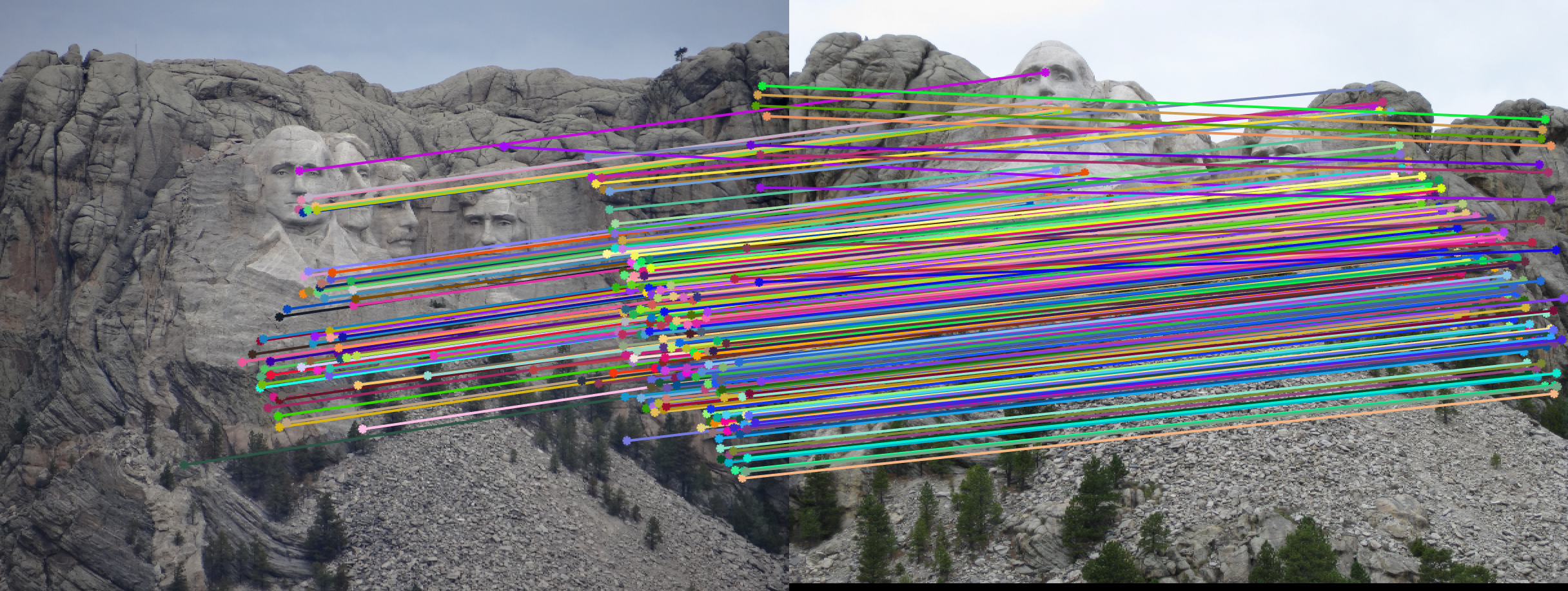
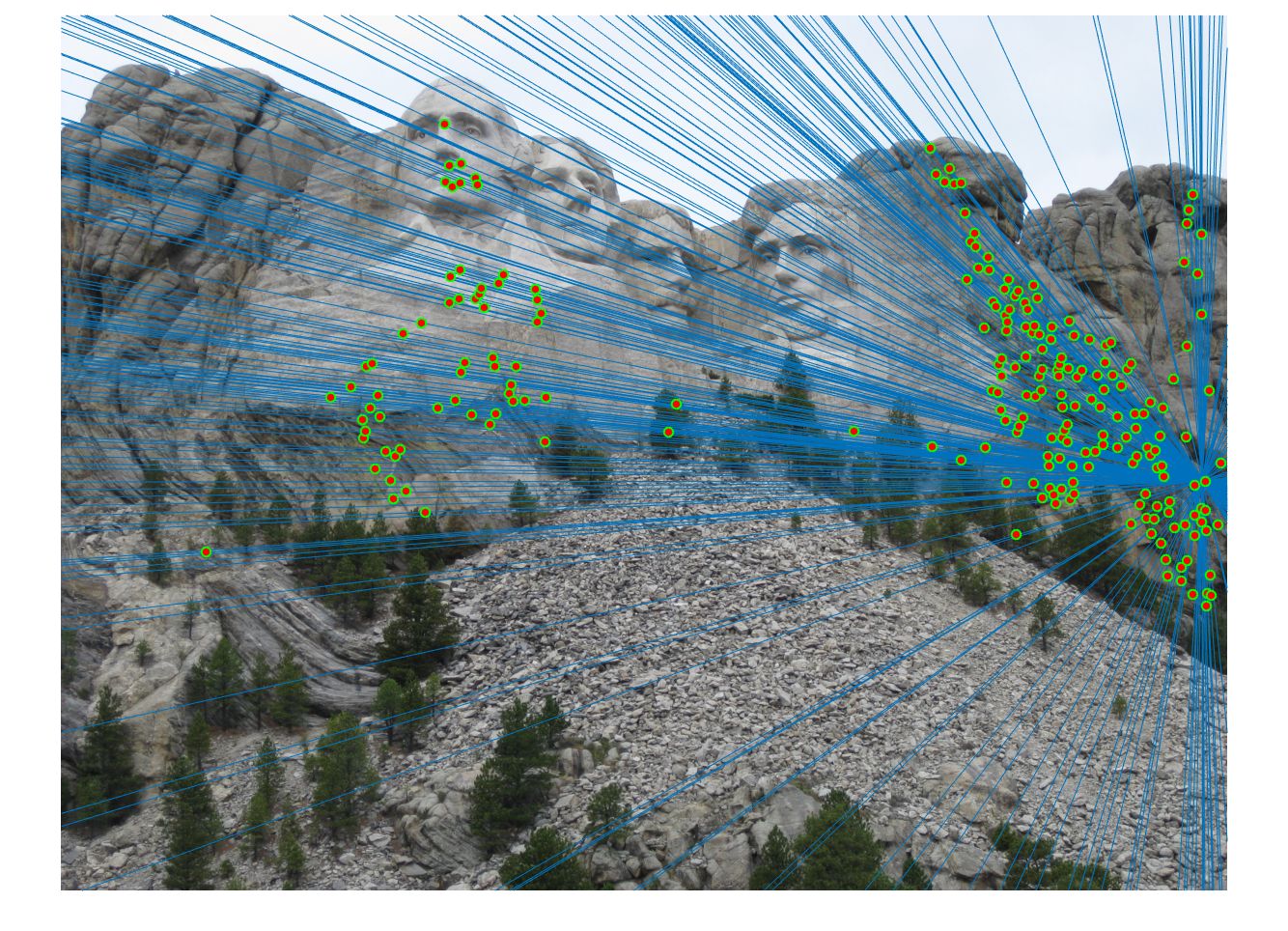
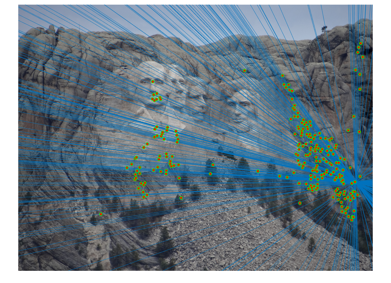
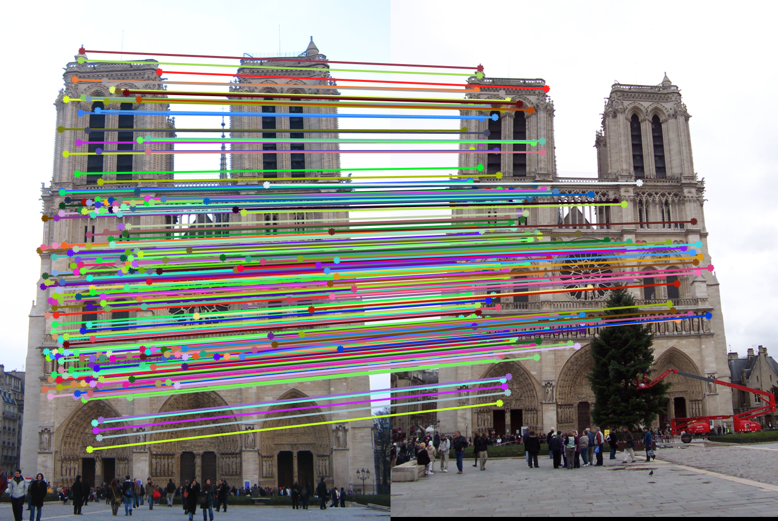
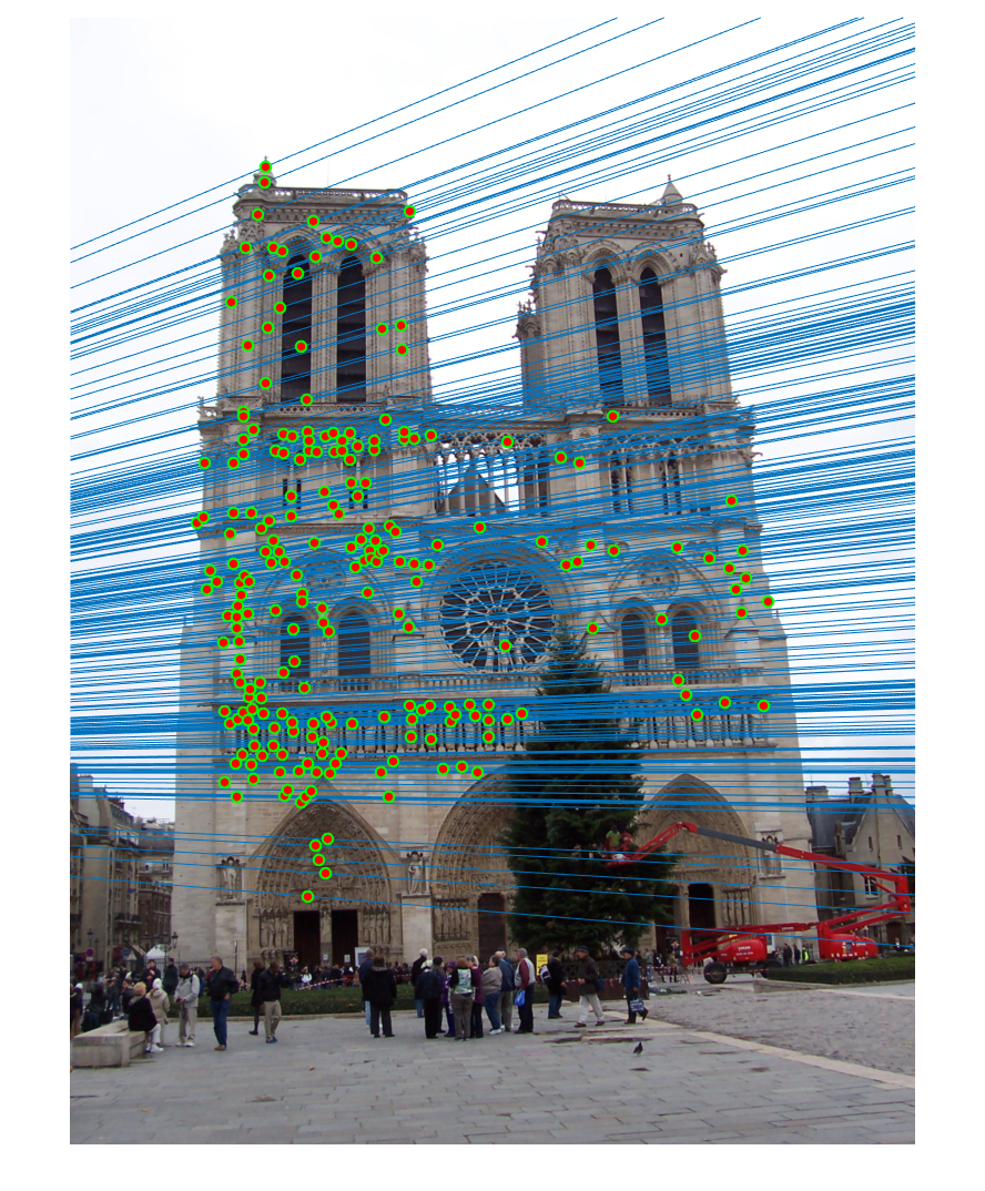
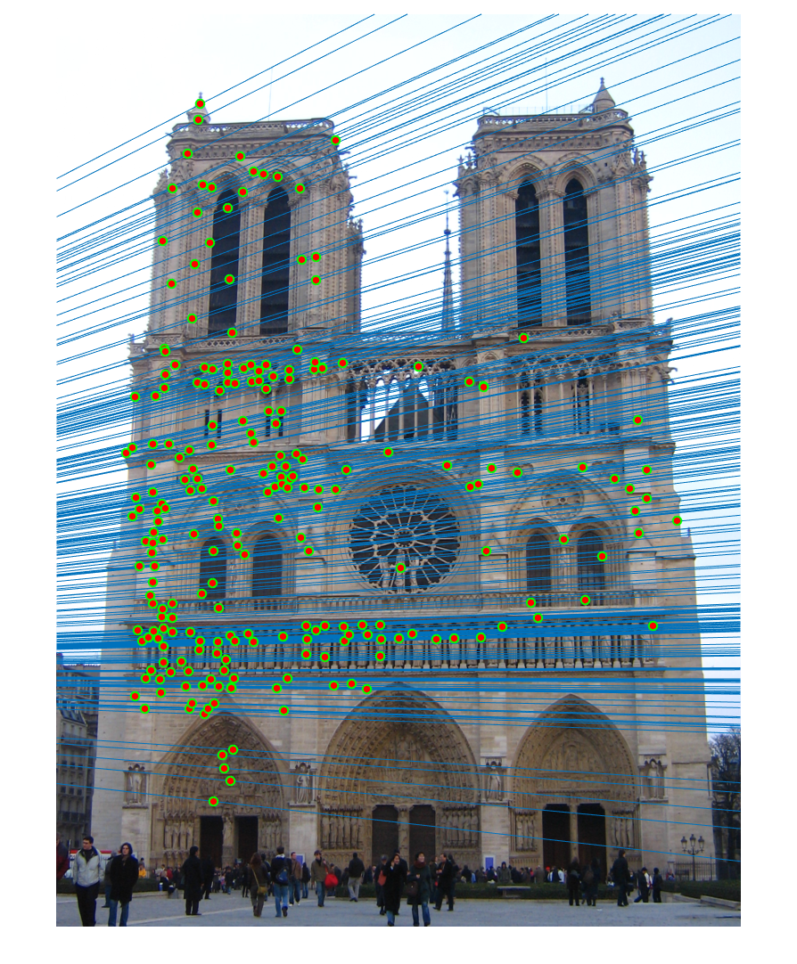
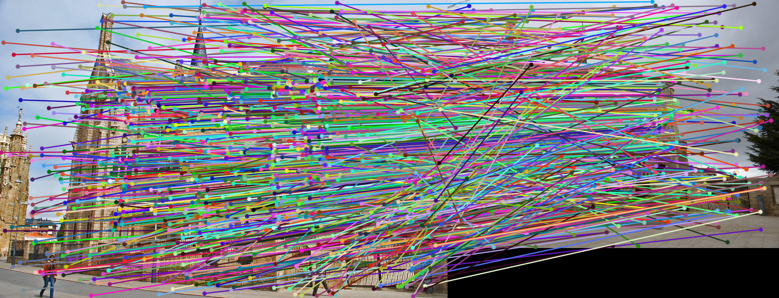
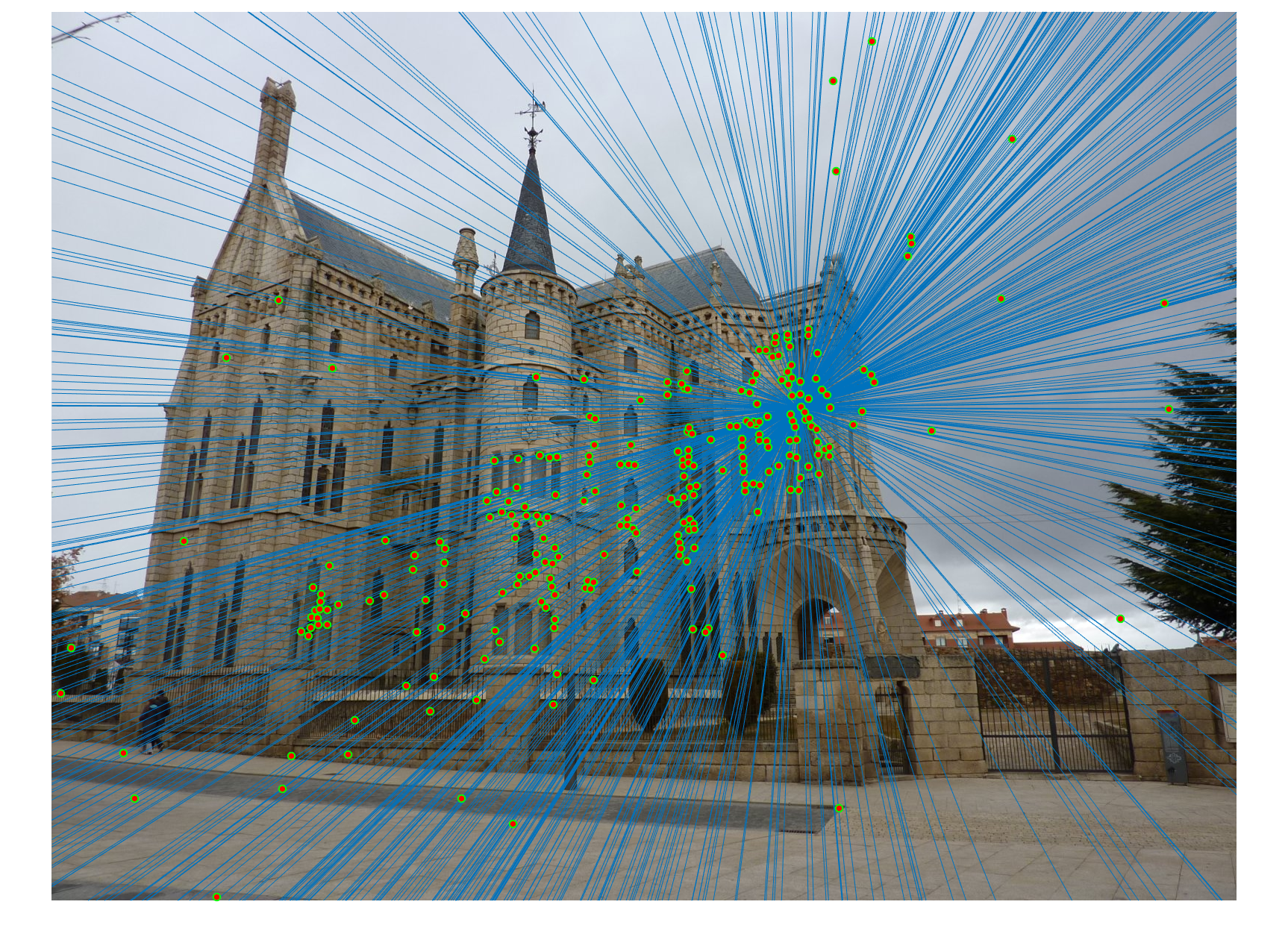
RANSAC to calculate fundemental matrix
We obtained perfect matching in Mount Rushmore example by doing RANSAC, probablistically eliminating effects of noise and outliers.
We obtained perfect matching in Notre Dame example.
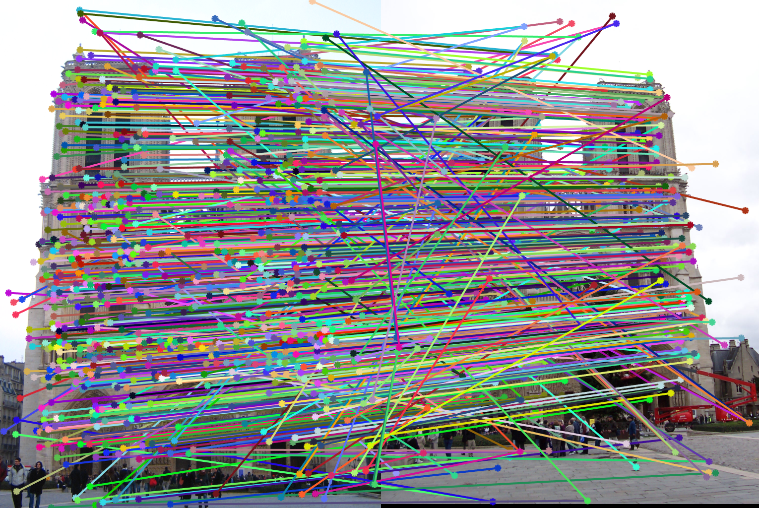
This one is harder, with lots of outliers. This is partially due to the difference in scale (image B is much smaller than image A, and thus the data points in image B are smaller in scale). The difference in scale led to large numerical error.
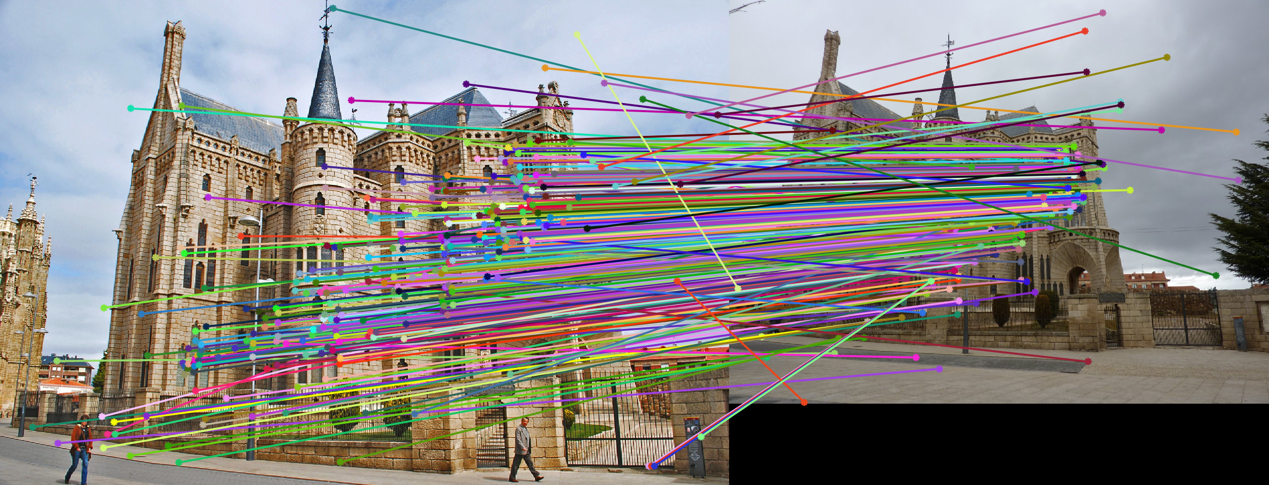
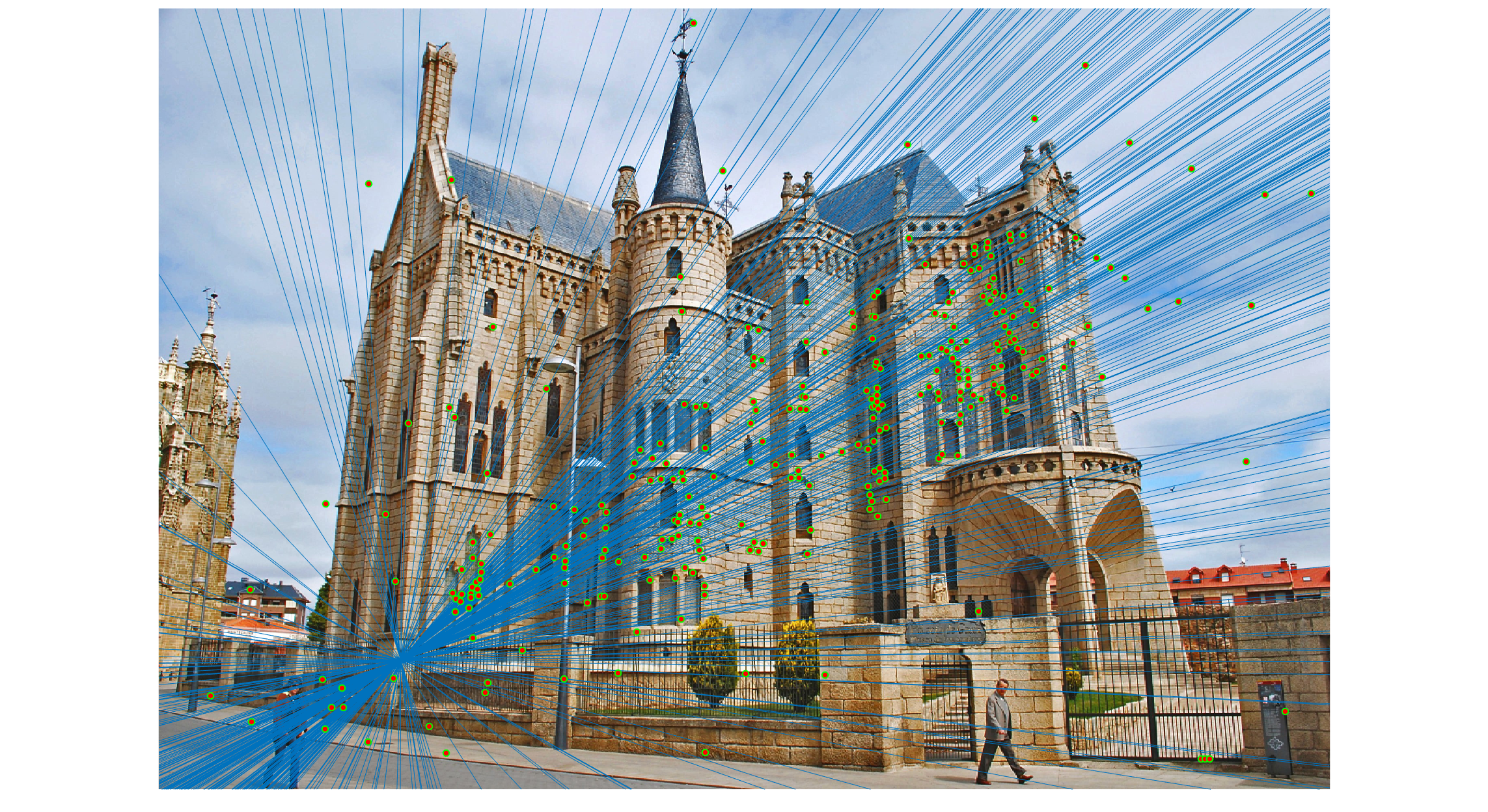
(Extra Credit) Normalized Points
After normalizing all data points, the accuracy increased because of less numerical error.