Project 3: Camera Calibration and Fundamental Matrix Estimation with RANSAC
This project implements techniques used in estimating camera parameters. The first method involves calibrating the cameras beforehand by estimating the projection matrix. Once we have an estimate, we can then retrieve camera parameters from the projection matrix. The project also explores cases where such estimates are not present, where we can estimate the fundamental matrix between an image pair to learn the relationship between the points and cameras. To do so, we use the 8-point algorithm with RANSAC. Finally, once we have a reliable estimate of the fundamental matrix, we can use it to remove spurious correspondence matches by check the epipolar constraints.
All results shown in this writeup will have the normalized coordinates feature enabled unless otherwise specified.
Part 1: Camera Projection Matrix
This part of the project tries to estimate the projection matrix of an image given 2D and 3D point correspondence pairs. The estimation is done by solving a linear system derived from definition. Since the projection matrix M is only defined up to scale, we fixed the scale by setting the last element of M to 1 (i.e. M_34 = 1). The following results was obtained for the normalized test case:
M =     0.7679   -0.4938   -0.0234    0.0067
       -0.0852   -0.0915   -0.9065   -0.0878
        0.1827    0.2988   -0.0742    1.0000

Total residual: <0.0445>
Estimated camera center: <-1.5126, -2.3517, 0.2827>
The results for the harder test set is shown below:
M =    -2.0466    1.1874    0.3889  243.7330
       -0.4569   -0.3020    2.1472  165.9325
       -0.0022   -0.0011    0.0006    1.0000

Total residual: <15.6217>
Estimated camera center: <303.0967, 307.1842, 30.4223>
Part 2: Fundamental Matrix Estimation
This part of the project estimates the fundamental matrix between two images using all correspondence points. Here, we assume that the given correspondence points are indeed reliable matches. The fundamental matrix is estimated by solving a linear system derived from the property transpose(x)*F*x' = 0. To address the issue of matrix scale, we use the same technique as the previous part where we set the last element of F to 1. Once we have solved for F, we use SVD to enforce the rank 2 restriction, where we remove the least significant eigenvalue.
Below are the results obtained from the provided test set:
F =    0.0000   -0.0001    0.0244
      -0.0001    0.0000   -0.1914
      -0.0006    0.2594   -5.2350
A potential issue with the aforementioned estimation technique is that the linear system becomes numerically unstable when we have large entries. This can arise quite frequenly as we multiply two coordinate values that are both large. To address this issue, coordinate normalization can be performed before the estimation. In this implementation, we first translate all points such that their mean is zero centered. Then we rescale the coordinates such that their averaged squared distance to the mean is 2. The normalization is implemented in this part but we will show the improvement in performance when it is more evident in the next part.
Part 3: Fundamental Matrix with RANSAC
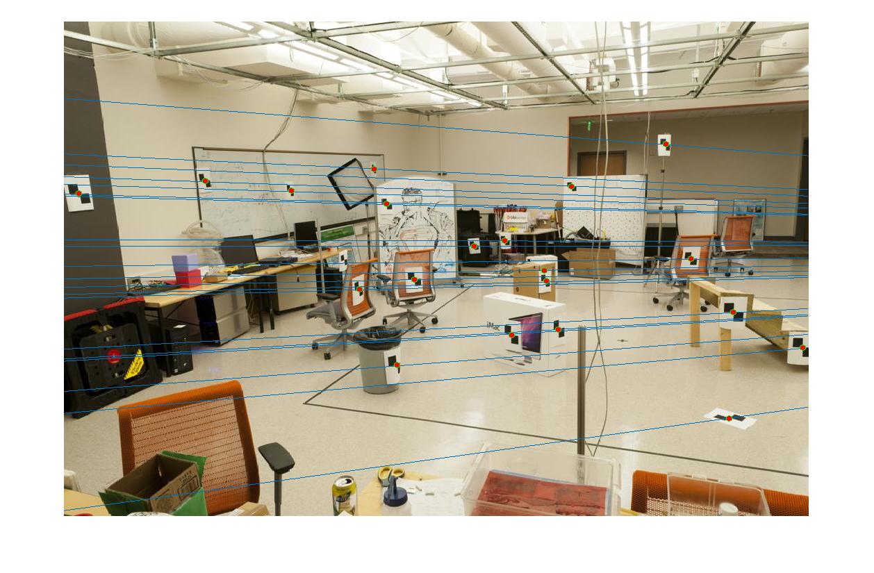
For real image sets, we cannot assume perfect point correspondences when calculating the fundamental matrix. In fact, the matching accuracy can be quite low as we have seen in the previous project. Hence, we fit the model using RANSAC, where we repeatly estimate the model using 8-point samples and pick the fit with the most inliers. To distinguish points between inliers and outliers, we take advantage of the fundamental matrix's property: transpose(x)*F*x' = 0. A correspondence pair is considered an inlier if this particular metric is less than 0.001.
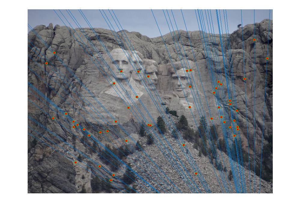
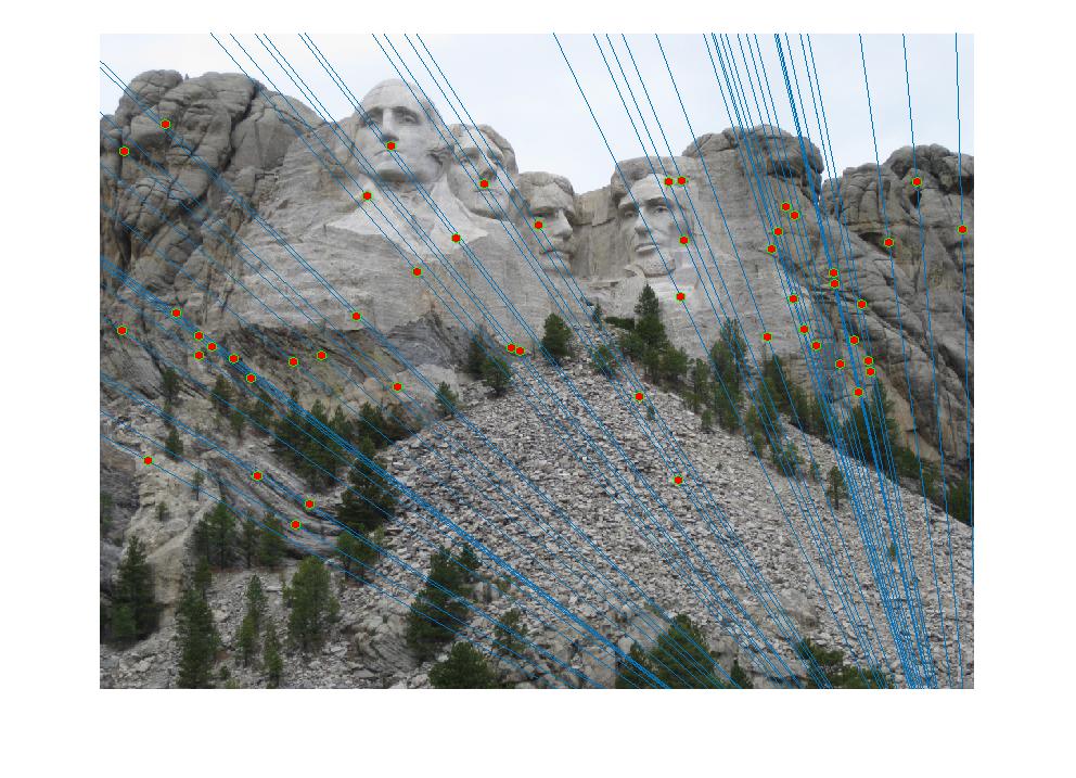
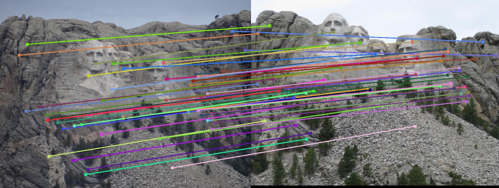
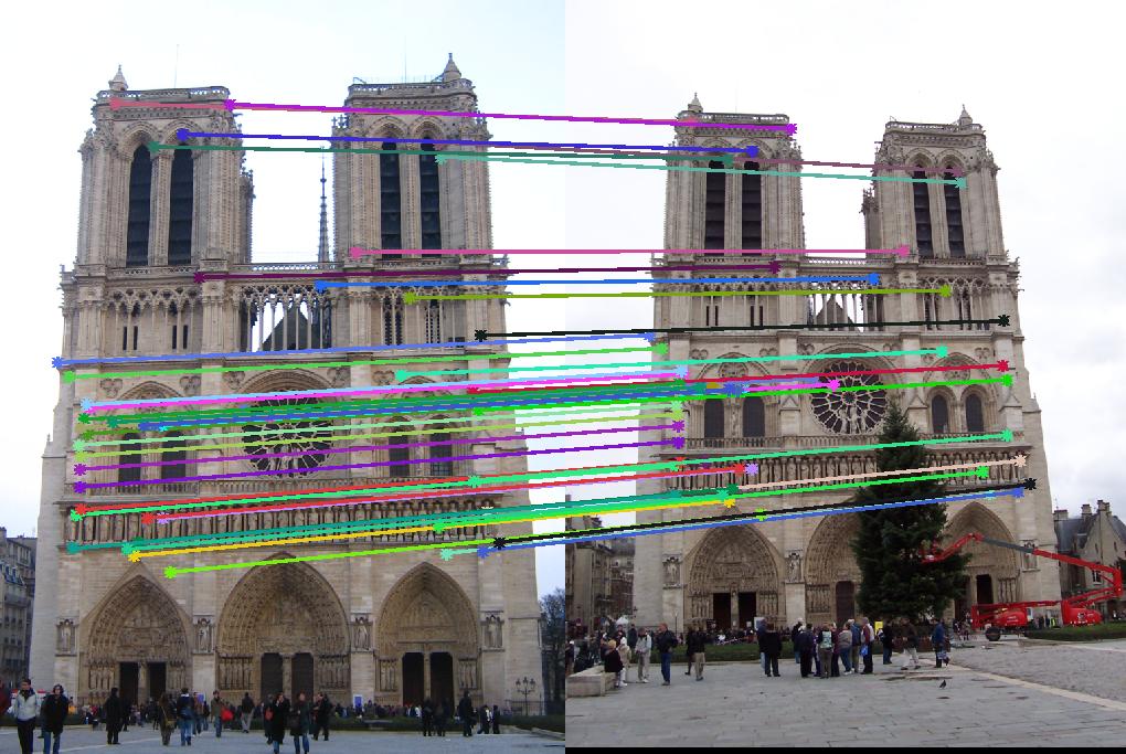
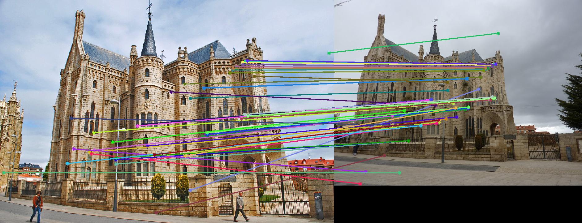
For all test cases shown below, we run the RANSAC process for 4000 iterations. We visualize the 50 most confident matches, where the confidence is determined by how close the threshold metric is to zero.
Below are the results for Mount Rushmore and Notre Dame:
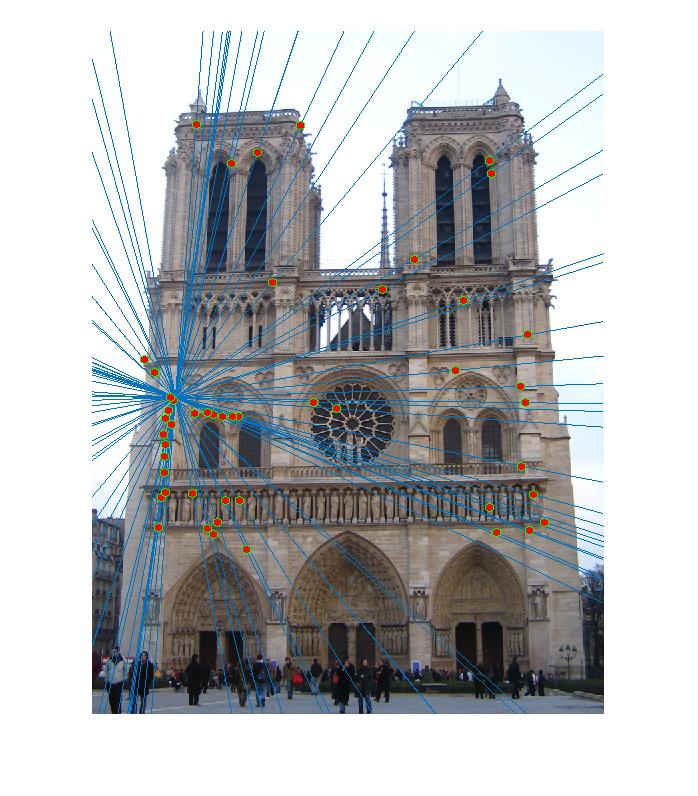
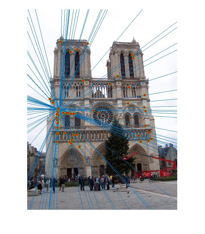
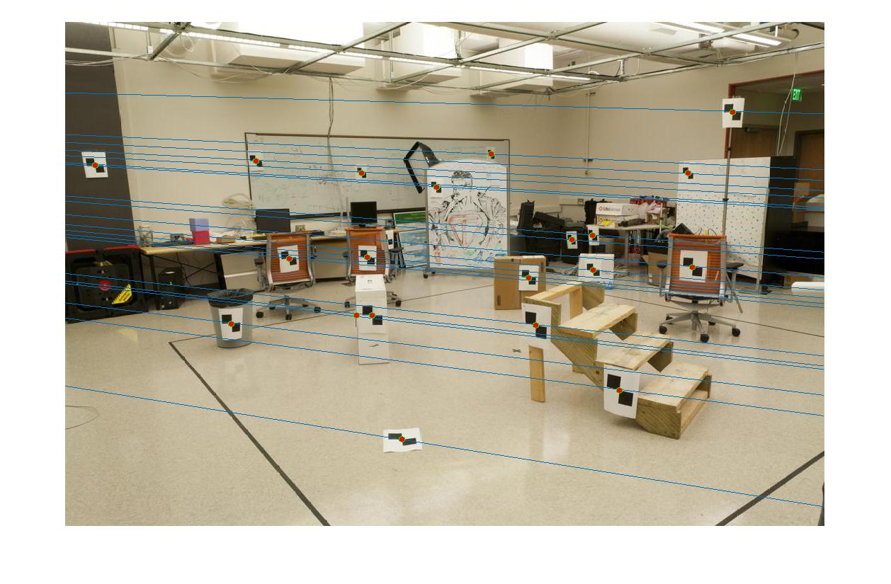
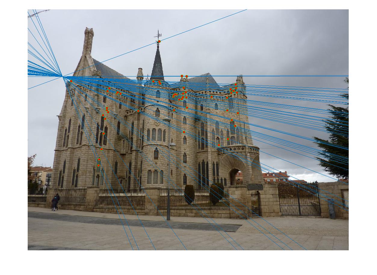
In the Episcopal Gaudi set, we will highlight the effect of coordinate normalization with respect to performance. The first set below shows the result without normalization and the next one with normalization. We can clearly see a significant improvement in performance.
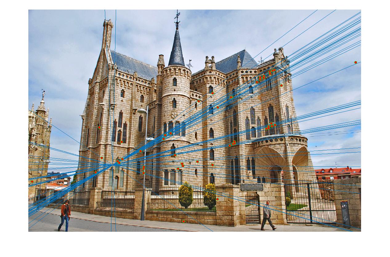
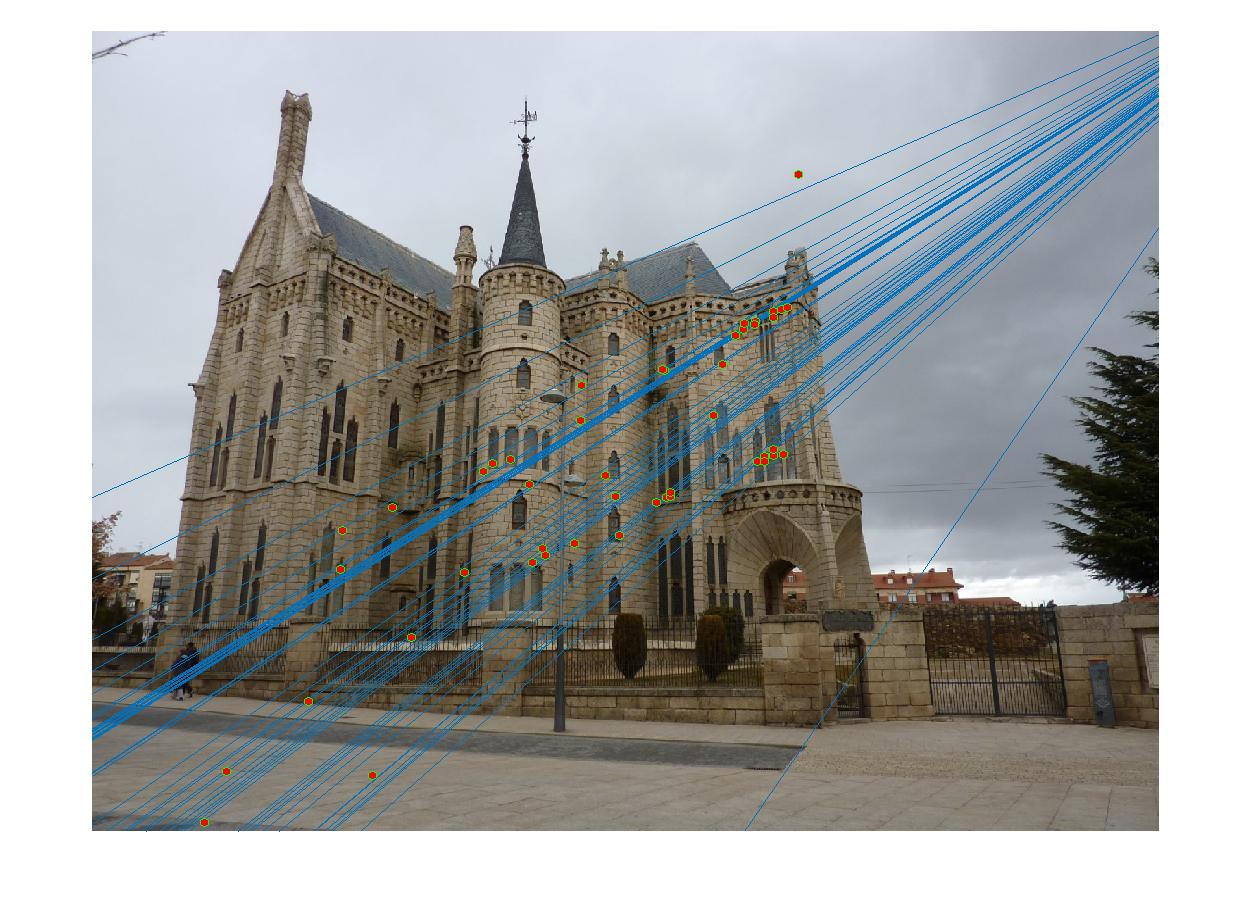
Epispocal Gaudi without coordinate normalization
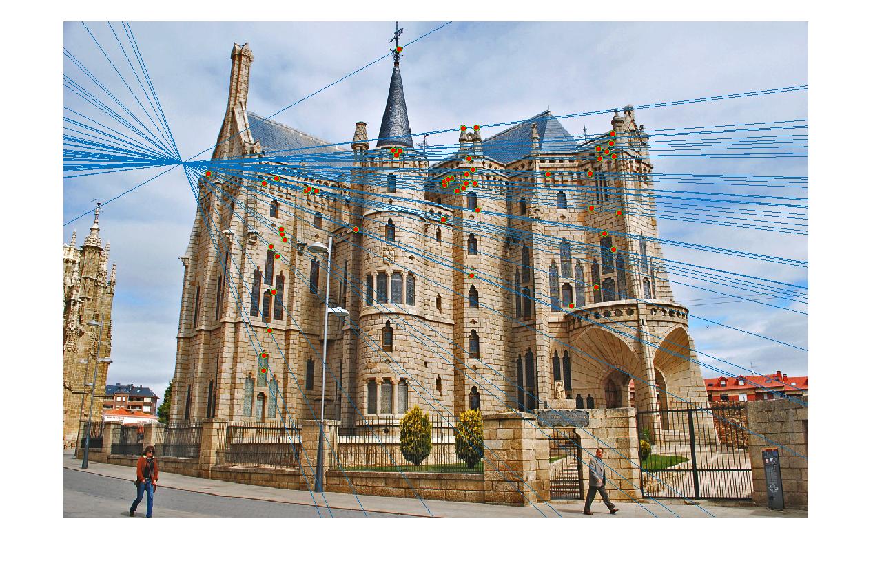
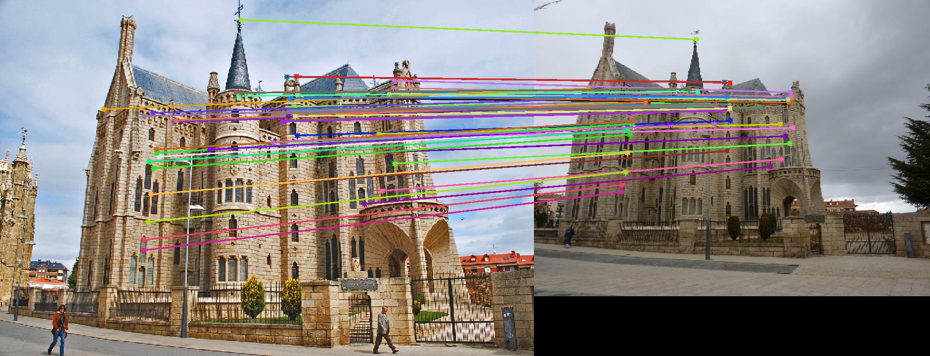
Epispocal Gaudi with coordinate normalization
In conclusion, the use of epipolar constraints allows us to obtain near perfect accuracy for previously intractable tasks.