Arjun Garg

Results of an example classifier

Tiny Images

Converting images into smaller, more manageable versions of themselves is a workable yet naive way to extract features. The way this works is by downsizing an image to a version with 16x16 pixels. These pixels are what define the features for each image. This allows for fast comparison, but it also ignores things like the high frequency values and spatial or brightness shifts.

K Nearest Neighbor

Using the given features for a set of training images and their matching labels, this algorithm works to classify a set of test images. For each image, it essentially compares its features against the features of each of the training images. It is then classified as the majority vote amongst the k most similar images from the training set. For k, I tried both 1 and 5. For k=1, I simply chose the class of the closest neighbor for the image. For 5, I used the code below to pick. I gave each neighbor a weight based on their distance from the image and added the weights for each class it could be, selecting the class with the highest weight. k=5 gave me a 1% increase in accuracy over k=1 while using Tiny Images, and a 4.4% increase on my main Bag of SIFT implementation.

map = containers.Map;
for j = 1:k
    word = train_labels{I(j)};
    if ~isKey(map,word)
        map(word) = 1/val(j);
    else
        map(word) = map(word) + 1/val(j);
    end
end
max = {'',0};
key = keys(map);
value = values(map);
for j = 1:map.Count
    if value{j} > max{2}
        max = {key{j},value{j}};
    end
end

Bag of SIFT

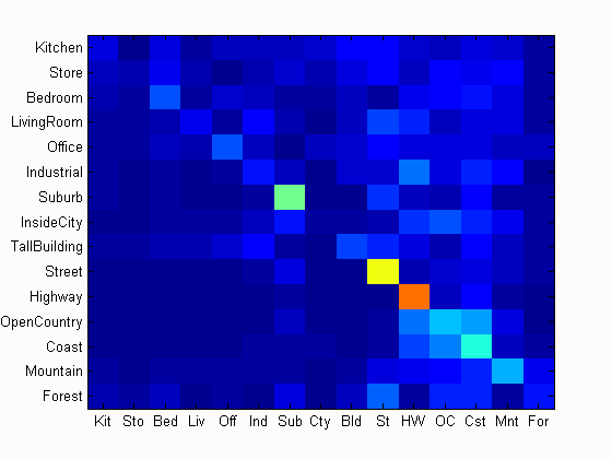
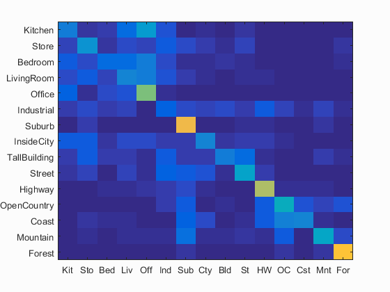
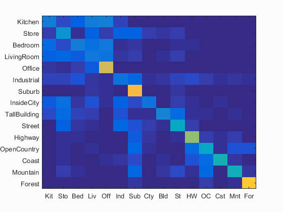
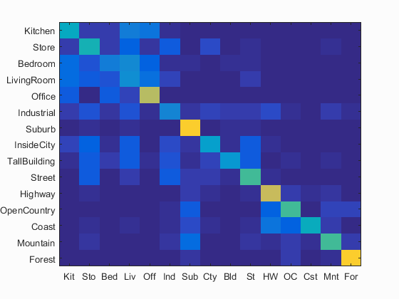
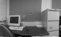
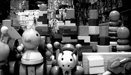
Bag of SIFT is another feature extraction method. However, this one is much more accurate and powerful. It extracts the SIFT features of each image to start with. For the training set, these sift features are clustered into k groups. The features of the test image are then dumped in these bins to develop a histogram for which types of objects the image contains. This histogram becomes the feature of the image. Below, we can see a few examples across decreasing step sizes. As the step sizes get smaller, the algorithm gets more accurate, but also a lot slower. The lowest accuracy is 39.5% and it goes all the way to 49.7%. I stuck with the second iteration as my step size to keep the time under 4 minutes.

Linear SVM

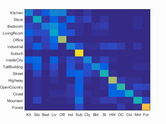
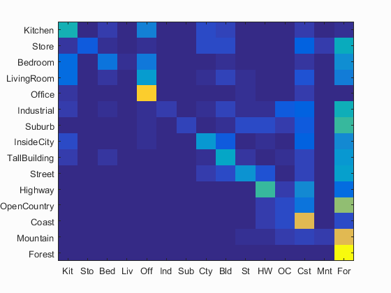
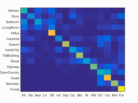
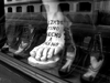
The linear SVM is another method of classifying images based on given features. This one trains a linear classifier so that it can apply itself to new features to classify them. linear SVMs are binary classifiers, so I had to train 15, one for each class. Each class' linear SVM sorted each image as either a member or not a member with a certain weight. The major adjustable input here was lambda, a value which determines how much weight is given to each change. This helps to keep the scaling of the effect of each training image on the classifier either high or low. This has a huge effect on accuracy. Here are some samples from a high lambda (10) and a low one(.000001). The best had an accuracy of 51%.

Results visualization for poorly performing recognition pipeline.

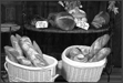
Accuracy (mean of diagonal of confusion matrix) is 0.261

Category name	Accuracy	Sample training images		Sample true positives		False positives with true label		False negatives with wrong predicted label
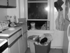
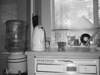
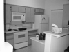
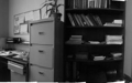
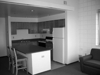
Kitchen	0.080					Industrial	Forest	Highway	Forest
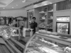
Store	0.040		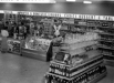			Office	TallBuilding	TallBuilding	Coast
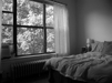
Bedroom	0.200					InsideCity	Store	OpenCountry	Mountain
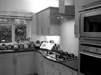
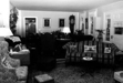
LivingRoom	0.100		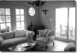			Office	Kitchen	Bedroom	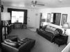Office
Office	0.190		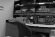			Mountain	Bedroom	Industrial	InsideCity
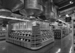
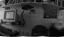
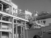
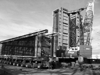
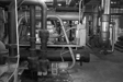
Industrial	0.130		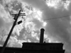			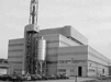LivingRoom	TallBuilding	InsideCity	Store
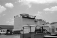
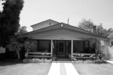
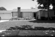
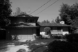
Suburb	0.470		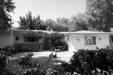			Coast	InsideCity	Kitchen	Street
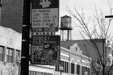
InsideCity	0.030					Suburb	Coast	TallBuilding	Store
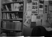
TallBuilding	0.180					Store	Forest	LivingRoom	Coast
Street	0.600					Kitchen	Store	Highway	Suburb
Highway	0.750					Suburb	Industrial	Coast	Mountain
OpenCountry	0.310					Forest	Kitchen	Suburb	Coast
Coast	0.400					Mountain	Mountain	InsideCity	OpenCountry
Mountain	0.290					Store	Bedroom	Kitchen	Forest
Forest	0.140					Mountain	Street	Suburb	Kitchen
Category name	Accuracy	Sample training images		Sample true positives		False positives with true label		False negatives with wrong predicted label