Project 4: Scene Recognition with Bag of Words
Scene recognition using bag of words used the idea of recognition of real world scenes that bypasses the segmentation and the processing of individual objects or regions. The procedure is based on a very low dimensional representation of the scene. The model generates feature descriptor for each image based on a multidimensional space in which scenes share membership in semantic categories. The initial work in this respect was introduced in 2001 with 8 scene categories. This was then modified to have 13 categories in the work published in 2005, and finally 15 categories later in 2006. In this project we use the 15 categories to perform scene recognition.
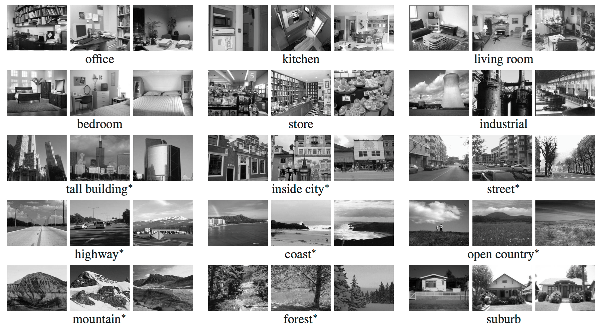
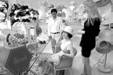
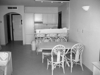
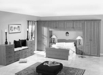
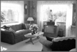
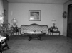
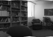
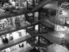
Figure 1: Example images from the scene category database.
In this project we are given a set of train images (with correct labels), and test images. We use various ways to represent the image, followed by two different ways to classify the images.
Representation of images:
- Tiny Image representation.
- Bag of SIFT representation.
- Bag of SIFT, with complementary GIST descriptors.
- Fisher Encoding Scheme.
- Kernel codebook encoding.
- Spatial Pyramid Representation.
The two different classification schemes used are:
- Nearest neighbour classifier.
- Linear SVM classifier.
In this project we run various combinations of the image representation schemes and classification techniques and provide a comparison in the performance of each of them.
I. Tiny Image and Nearest Neighbours:
Tiny images uses image downsizing, and using this downsized image as the representation of the image. An important benefit of working with tiny images is that it becomes practical to store and manipulate datasets orders of magnitude bigger than those typically used in computer vision. In this project we compare the results of the following image representations. For tiny image representtion, the image is resized using imresize to the target size. This resized image is then reshaped to a row vector. This row vector is our image's representation. We represent all the train and test images the same way.
- 16x16 tiny image representation
- 32x32 tiny image representation
We use nearest neighbour classification as our classification technique. Each test vector is then assigned to a class by considering k nearest neighbours. The image is assigned to highest common class among the nearest neighbous considered.
Parameters considered: size of tiny image, number of nearest neighbours.
Figure : Examples of nearest neighbour classification using k = 5 and k = 8.
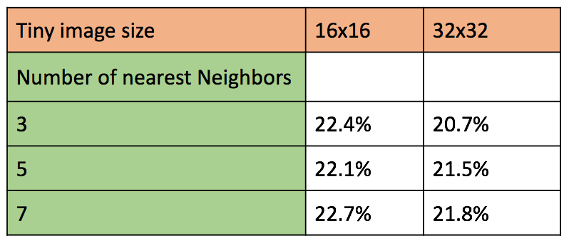
Figure 2a: Table of accuracies for different tiny image sizes and number of nearest neighbors.
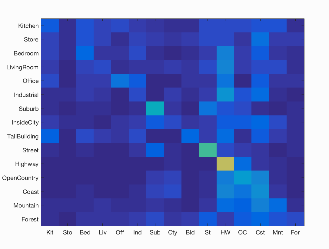
Figure 2b: Confusion matrix of best accuracy = 22.7% with image size 16x16 and 7 nearest neighbors.
Analysis of results for Tiny Image and Nearest Neighbours:
The free parameters in this combination of image descriptor and classifier are the tiny image size, and number of nearest neighbours considered for test image classification.
- We observe that with increase in tiny image size, the accuracy goes down slightly. Although this decreas is too slight (1%) to be considered stable, we see consistence in the decrease through all test cases. This can be analyzed as a result of increase in specificity of features. Larger the image feature, more information wil be captured in the tiny image, thus making slight change in train and test image to be further apart from each other in the feature space, thus increasing the number of false negatives.
- The second free parameter is the number of nearest neighbours considered for K-nn classifier. Here, we observe a fractional increase in accuracy with increase in number of nearest neighours. This trend stops beyond 7 nerest neighbours, where the accuracy was observed to decrease drastically (too low to be reported).
II. Bag of SIFT with nearest neighbors classification.
In Bag of SIFT we use dense scale invariant feature transform to obtain the feature descriptors. Once we obtain the descriptors, we obtain a histogram based on its closeness to a set of predefined vocabulary. We first build this vocabulary by using the train dataset. We build the vocabulary by generating sift descriptors of train dataset, randomly sampling few thousand descriptors from these,and clustering them. We use kmeans clustering to cluster the sift descriptors into a fixed number of clusters. In our project, we have used 200 clusters. With lower number of clusters we observed a slight drop in the accuracy of all test cases. The means obtained by kmeans clustering is saved in a vocabulary named 'vocab.mat'.
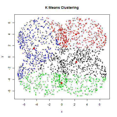
Figure : Example of Kmeans clustering. The red points are means found after clustering.
Once we have our vocabulary in place, we build our image feature vector by generating a histogram of the count of sift features closest to each of the means in our vocabulary. Such image representation is generated for all the test and train data. We then use nearest neighbours to assign classes to the test vectors, and calculate accuracy based on ground truth.
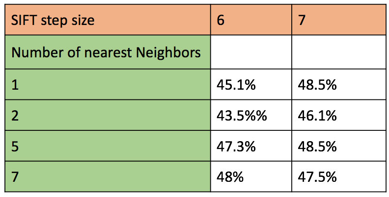
Figure : Accuracy of various combination of parameters for SIFT representation and classification using k-nearest neighbours with k = 5 and k = 8.
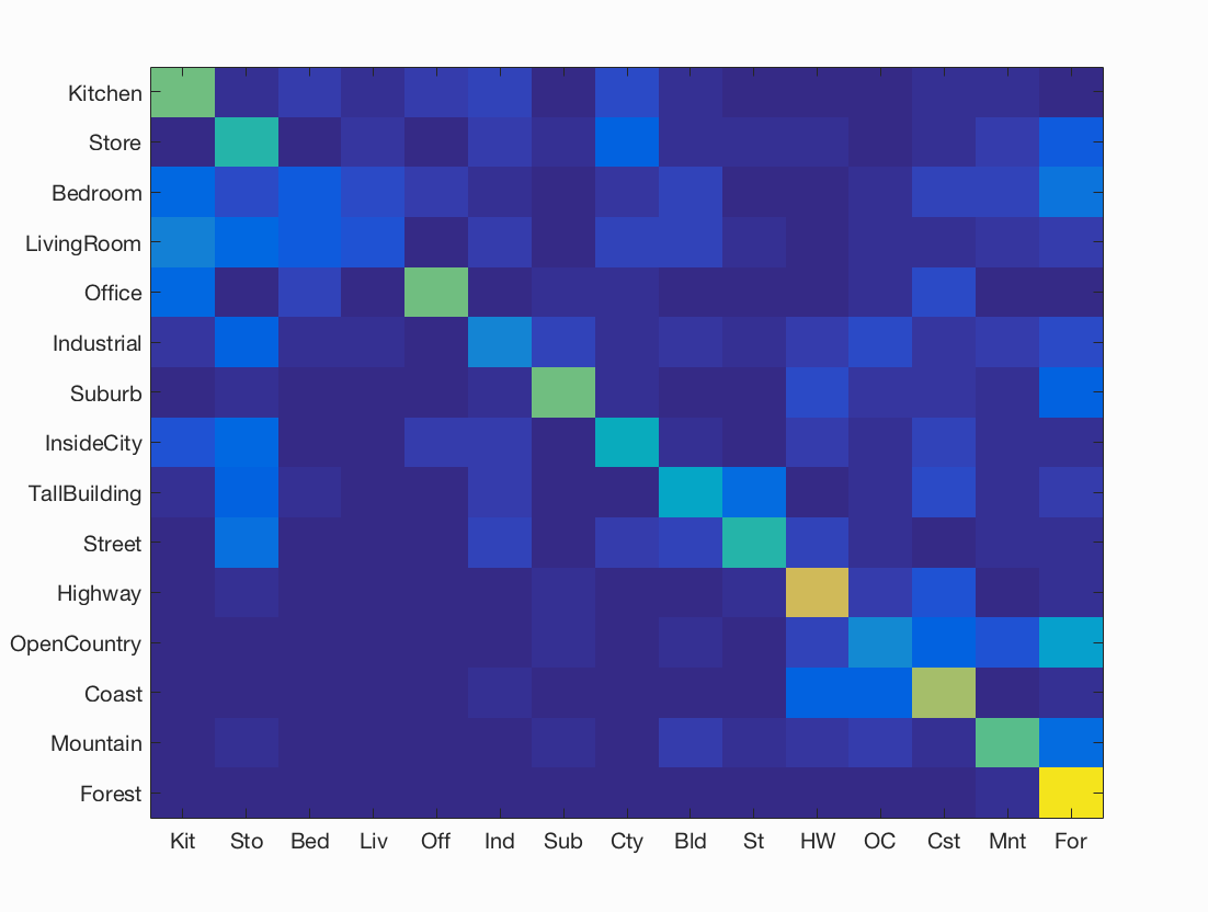
Figure : Confusion matrix for best accuracy = 48% obtained using sift step size = 6, and 7 nearest neighbours.
Analysis of results for Bag of SIFT with nearest neighbors classification:
The free parameters in this combination of image descriptor and classifier are the SIFT step size size, and number of nearest neighbours considered for test image classification.
- The SIFT step size is present in two cases. Once while building vocabulary, and the second time while generating image representation of test and train images. In both the cases, we observed that lower the step size, higher was the execution time. We considered for step size of 6 and 8, and observed better accuracy for step size of 8. This is because with lower step size, we have more densely packed SIFT features, which with nearest neighbour classifier leads to considering too closely spaced features, thus giving a poor representation. There will be too many feature vectors ner each other which will throw off the balance of getting good enough points of both classes for correct classification.
- For building vocabulary, we tried with different sized feaature sizes (or vocab_size) vocabulary like 50, 200 and 300. The best accuracy was obtained with 200 clusters centers. The run time for creating the vocabulary was lower with picking random sift vectors, and accuracy increased marginally (~1 to 2%). This can be reasoned as too many sift features will make it less likely to have clearly separable clusters, thus throwing off the mean of each cluster. Thus we use vocab with vocab-size 200 for the rest of test combinations with SIFT.
- The second free parameter is the number of nearest neighbours considered for K-nn classifier. Here, we observe a fractional increase in accuracy with increase in number of nearest neighours. This trend stops beyond 7 nearest neighbours, where the accuracy was observed to decrease drastically (too low to be reported).
IIIa. Bag of SIFT with Linear SVM.
In Bag of SIFT we use dense SIFT to transform the test and train images and obtain their feature descriptors. We build a histogram of count by using a pre-built vocabulary. The histogram is built by finding the closest vector in the vocabulary to each of the test and train images's SIFT descriptor.
Once we have our SIFT feature for each image in train and test dataset, we classify it using linear SVM. Linear SVM generates a linear binary classifier. Since we have 15 classes, we have to perform 15 one vs all classification. With this, we get 15 binary classfiers. The linear classifiers are of the form WX + B = class. Since it is a binary classifier, the class is either +1 or -1 denoting belongs to class, and does not belong to class respectively. W is the matrix of weights, and B is the vector of weights. An example of linear classifier is shown in figure below.
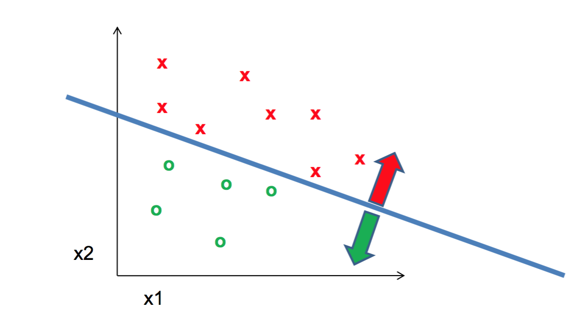
Figure : Example of linear classification using one vs all SVM.
These classifiers are generated using train images. The same classifiers are used on each of the test images to calculate their score using WX + B where W and B are the same as calculated using the train images. Since it is a one vs all classification, the final classification of each test image is dependent on the score of WX + B of all classes. the highest scoring classifier is the final class assigned to the test image.
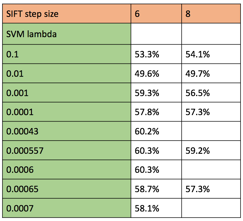
Figure : Accuracy of various combination of parameters for SIFT representation and classification using SVM
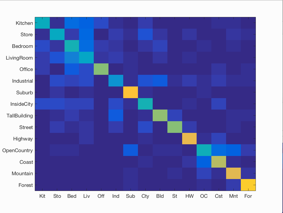
Figure : Confusion matrix for best accuracy = 60.2%% obtained using sift step size = 6, and lambda = 0.000557.
Analysis of results for Bag of SIFT with Linear SVM:
The free parameters in this combination of image descriptor and classifier are the SIFT step size, and lambda which is the regularization parameter that serves as a degree of importance that is given to miss-classifications. We performed the experiment with fast parameter in vl_dsift, and without it. with 'fast' the runtime was much less, and accuracy was slightly better. This may be due to the fact that fast vl_dsift performs denser sift description extraction.
- The SIFT step size is present in two cases. Once while building vocabulary, and the second time while generating image representation of test and train images. In both the cases, we observed that lower the step size, higher was the execution time. We considered for step size of 6 and 8, and observed better accuracy for step size of 6, unlike above. This is because with lower step size, we have more densely packed SIFT features, which with SVM classifier gets a better confirmation that a particular side of the linear classifier is positive or negative. With sparse data-points, it is difficult to create a clear boundary between the two classes. As we get better results with SIFT Step size 6 with SVM classification, we use only this step size for the rest of the test combinations. For SIFT vocabulary, We maintain the SIFT step size of 6, with vocab size of 200 (number of kmeans cluster) as we observed that gives us consistent results.
- The second free parameter is the regularization parameter of SVM classifier. Here we try a number of values ranging from 1 to 0.0001. We find comparable accuracies for lambda = 0.0004, 0.000557 and 0.0006. Higher the lambda, each miss-classification costs too much thus resulting in more false negatives. On the other hand, lower lambda results in too much lax towards miss-classifications thus resulting in more false positives. Thus we use a range of lambdas around the ones we got with this test for the remainder of test combinations using SVM classification.
- We observe a sharp increase in accuracy from nearest neighbour classification to SVM classification. This is because knn classifier is more prone to over fitting, and does not have a concept of soft classifier with regularization for miss-classifications far away from the boundary.
EXTRA CREDIT
IIIb. Analysis of different vocabulary size for Bag of SIFT with Linear SVM:
For extra credit, we train vocabulary of different sizes using SIFT descriptors. For analysis that can be comparable, we use the SIFT step size = 6, and lambda for SVM clssifier = 0.000557 as these correspond to the best accuracy with Vanilla SIFT and SVM vocab size 200. The accuracies we observe are presented in the table below. On analyzing it, we observe that for lower codebook sizes, the accuracy falls steeply below the accuracy for corresponding step size and svm regularization parameter.
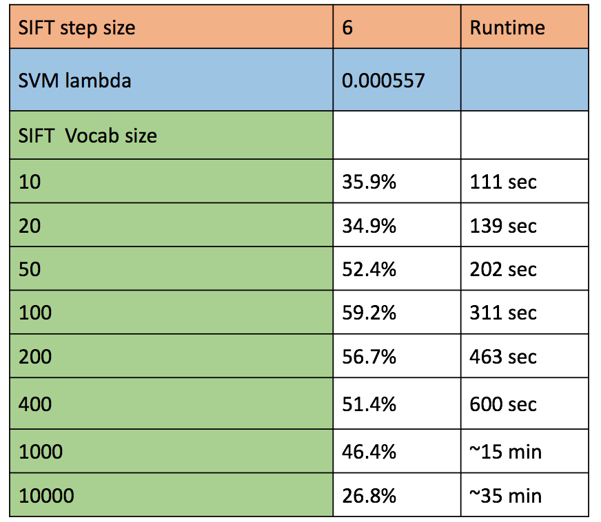
Figure : Accuracy of various vocab sizes of SIFT descriptors and classification using SVM.
IV. Spatial Pyramid Representation with SVM classification.
In spatial Pyramid, we take into account the spatial information about an image as well. Here we divide the image into four or sixteen smaller images, and take individual histograms for each of them. This is shown in the figure below. The histograms are then weighted as 1/4 times for level 1, and 1/16 times for level 2.
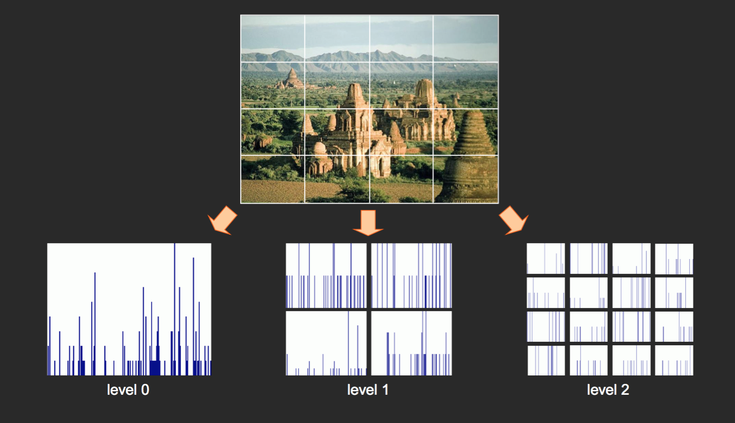
Figure : Example of level 0, 1 and 2 of the spatial pyramid.
In this method of image representation, we take into account the histograms of gradients in different parts of the image and thus retain some information of spatial arrangement. on weighing the different histograms, they must be combined. THe combination can be done in many ways like concatenating, stacking or adding. In this project, we add the weighted histograms to finally have one histogram per image.
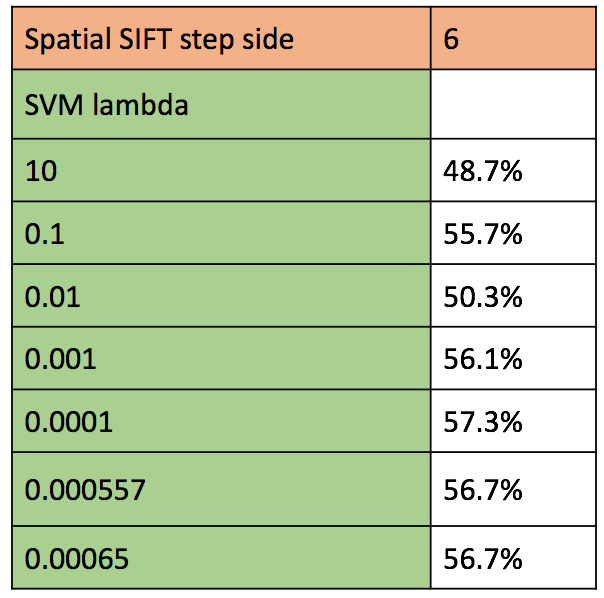
Figure : Accuracy of various combination of parameters for SIFT representation and classification using SVM
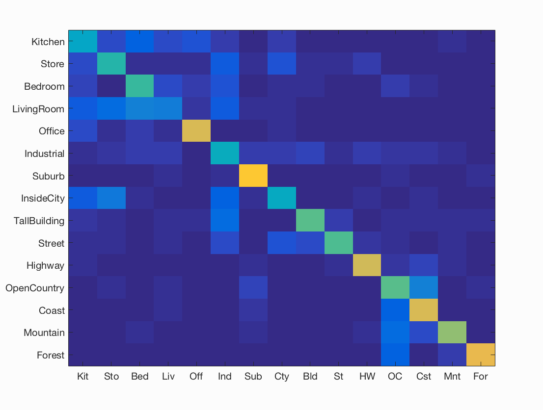
Figure : Confusion matrix for best accuracy = 60.2%% obtained using sift step size = 6, and lambda = 0.000557.
Analysis of results for Spatial Pyramid Representation with SVM classification:
The free parameters in this combination of image descriptor and classifier are the SIFT step size size, and lambda which is the regularization parameter that serves as a degree of importance that is given to miss-classifications. Additionally, we also have the free parameters associated with spatial pyramid viz., number of levels, weight associated with each level, and method of combination of the levels.
- We maintain the SIFT step size of 6, with vocab size of 200 (number of kmeans cluster) as we observed that gives us better results with SVM classifier.
- The second free parameter is the regularization parameter of SVM classifier. Here we try a number of values ranging from 1 to 0.0001. We find comparable accuracies for lambda = 0.0001, 0.000557 and 0.00065. Higher the lambda, each miss-classification costs too much thus resulting in more false negatives. On the other hand, lower lambda results in too much lax towards miss-classifications thus resulting in more false positives.
- In our project we have used three levels to build a spatial pyramid. The base level 0 considers the entire image as one unit. The first level 1 divides the image into 4 equally sized blocks and build one histogram for each. Each of these histogram is weighted with 1/4. The second level, level 2, divides the image into 16 sub-images, and builds 16 histograms. Each of these is weighted as 1/16.
- We observe a slight decrease in accuracy for spatial SIFT features. The reason for this can be the small size of original images, which results in very little new information being added due to smaller sub-images of level 2. The runtime of this test is considerably high as conpared to the others.
V. GIST Descriptor with Linear SVM classification.
SIFT descriptors are local descriptors, i.e. they provide feature descriptors of local patches of image around corner points. GIST is a global descriptor. Intuitively, GIST summarizes the gradient information (scales and orientations) for different parts of an image, which provides a rough description (the gist) of the scene. Thus, in this project we use GIST descriptor with SIFT. There are various ways of combining both the descriptors viz., adding them, weighing them while classifying, etc. In this project we concatenate them horizontally such that they enhance the classification accuracy of vanilla SIFT.
The parameters that we can alter in GIST is number of orientations per scale, number of blocks, and pre filtering. In order to get 128 length feature vector like SIFT, we use a total of 32 scales, 2 blocks, and filter size 4. The other free parameters are those related to linear SVM classification. The cost of miss classified data points within the support vector margin (denoted my lambda) is tuned with values ranging from 10 to 0.00001. A table of accuracies obtained for different combinations of free parameters is shown below.
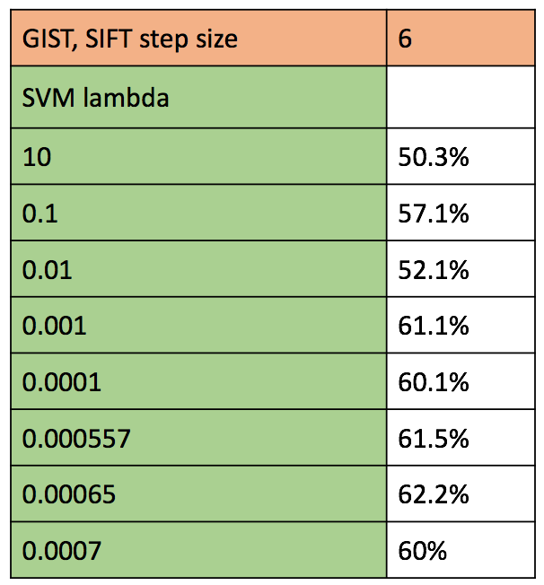
Figure : Accuracy of various combination of parameters for concatenated GIST - SIFT representation and classification using SVM
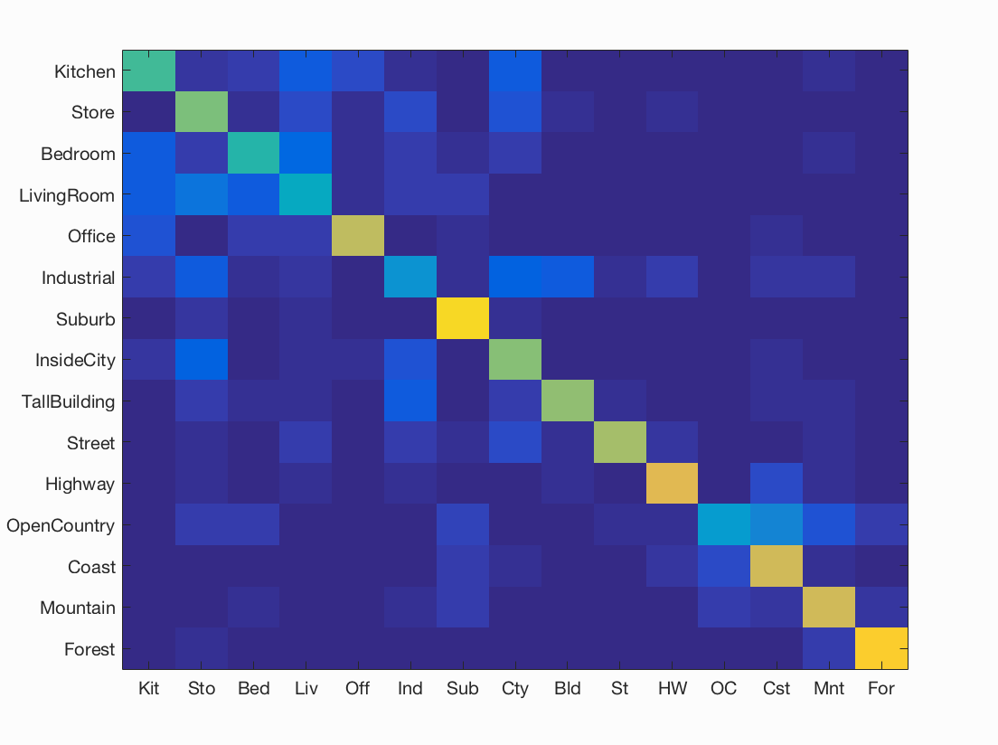
Figure : Confusion matrix for best accuracy = 62.2%% obtained using sift step size = 6, and lambda = 0.00065.
Analysis of results for GIST Descriptor with Linear SVM classification:
The free parameters in this combination of image descriptor and classifier are the SIFT step size size, and lambda which is the regularization parameter that serves as a degree of importance that is given to miss-classifications. Additionally, the parameters that we can tune in GIST is number of orientations per scale, number of blocks, and pre-filtering.
- We maintain the SIFT step size of 6 with vocab-size (number of kmeans cluster) of 200 as we observed that gives us better results with SVM classifier.
- The second free parameter is the regularization parameter of SVM classifier. Here we try a number of values ranging from 1 to 0.0001. We find comparable accuracies for lambda = 0.0004, 0.000557 and 0.0006. Higher the lambda, each miss-classification costs too much thus resulting in more false negatives. On the other hand, lower lambda results in too much lax towards miss-classifications thus resulting in more false positives.
- In order to get 128 length feature vector like SIFT, we use a total of 32 scales, 2 blocks, and filter size 4. There are various ways of combining the GIST descriptor with SIFT descriptors. In this project, we have horizontally concatenated them to get a higher dimension representation for each image.
- We observe a considerable increase in accuracy from vanilla SIFT to SIFT+GIST. This is because the feature size of each image is larger now, which adds global information of the image to our image representation. More the information, better will be the features, resulting in better recognition.
VI. Feature encoding using Fisher Vector.
Till now we have used descriptors like SIFT or GIST in its raw form. From here on we see various coding schemes that encode the feature vector and help us obtain a an image representation. Fisher Vector is an image representation obtained by pooling local image features. A Gaussian Mixture Model is found that fits the distribution of image descriptors like SIFT descriptors. The GMM associates each image vector to a mode k in the mixture. a Gaussian Mixture Model can he represented with Mean, Covariance and Priors. This is shown in the figure below. Thus, we save these three parameters as means.mat, covariances.mat and priors.mat which is loaded and used to apply on the test and train images. This helps us generate a Fisher vector, which is our final image representation of a single image.
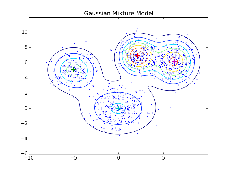
Figure : Example of Gausian Mixure Model clustering. The means of each cluster is shown as a '+'.
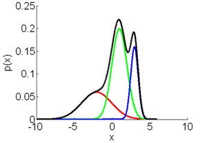
Figure : Example of how the constituting Gaussian distributions are seen in a GMM.
Classification is done using linear SVM. In this method, the fisher vectors are the image representations of the test and train images. After we have found both these Fisher vectors, we train a linear SVM to obtain the weights and offset of a classifier for each class. As a linear SVM is binary classifier, we train 15 classifiers, one for each of the categories. The test images are scored based on the results of the trained classifier. In Fisher, the number of clusters in Gaussian Mixer model is tuned to find the model which gives us best accuracy as shown the the table of accuracy below.
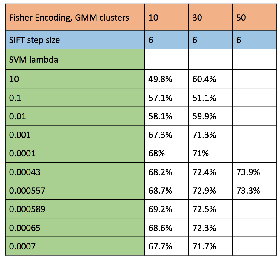
Figure : Accuracy of various combination of parameters for SIFT representation and classification using SVM
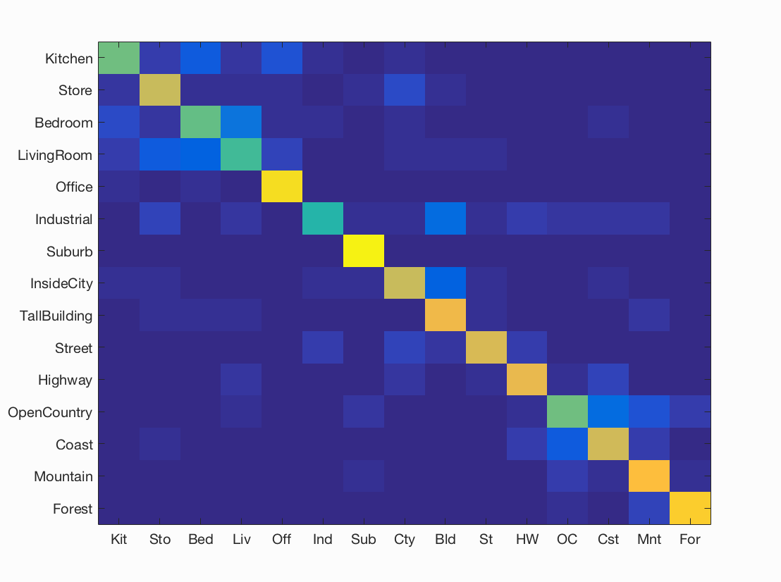
Figure : Confusion matrix for best consistent accuracy = 72.9%% obtained using GMM cluster size 30, sift step size = 6, and lambda = 0.000557.
Analysis of results for Feature encoding using Fisher Vector:
Using this image representation technique, we switch gears slightly from the previous test cases. Here Fisher requires Gaussian mixture models. This requires generating a GMM. The free parameters in this are number of clusters. As we cluster SIFT features to GMM, we have the free parameters of SIFT as well. We continue to use SVM classifier, which gives us regularization parameter to be tuned.
- For SIFT, we maintain the SIFT step size of 6, as we observed that gives us consistent results.
- The next free parameter is the number of clusters of GMM while building the vocabulary. The test cases executed involve 10, 30 and 50 clusters. With respect to runtime, 50 clusters took extremely long to cluster in comparison to 10 and 30 clusters. As expected, we find better results with more clusters. This is because, higher the number of clusters, more accurately the model will be able to fit to the train data. We expect the accuracy to reduce at one point of increased cluster size due to over fitting to train data. Due to high runtime, 50 clusters is not a viable result although it gives better accuracy. 30 clusters was the sweet spot with respect to accuracy and run-time. We hit the highest overall accuracy among all techniques in Fisher enoding. This may be due to the large size of feature vector, with all useful information. As suggested in the Paper, PCA was applied to the Fisher vectors to reduce the runtime/remove low information data. There was not observable reduction in runtime, as vl_dsift is extremely efficient. The accuracy, on the other hand, dropped slightly.
- The next free parameter is the regularization parameter of SVM classifier. Here we try a number of values ranging from 10 to 0.0001. We find comparable accuracies for lambda = 0.00043, 0.000557, 0.000589 and 0.00065. Higher the lambda, each miss-classification costs too much thus resulting in more false negatives. On the other hand, lower lambda results in too much lax towards miss-classifications thus resulting in more false positives.
- We observe a sharp increase in accuracy from vanilla SIFT to Fisher Encoding. This is because the feature size of each image is larger now, with smart encoding using gaussian mixture models. More the useful information, better will be the features, resulting in better recognition.
VII. Kernel Codebook Encoding
Kernel Codebook encoding is a soft assignment technique that overcomes the hard assignment of codewords in the vocabulary to image feature vectors using SIFT. The hard assignment of codewords to image features overlooks codeword uncertainty, and may label image features by non-representative codewords. The codebook approach merely selects the best representing codeword, ignoring the relevance of other candidates. Here we apply techniques from kernel density estimation to allow a degree of ambiguity in assigning codewords to image features. In our traditional histogram words using vocabulary, a robust alternative to histograms for estimating a probability density function is kernel density estimation. Kernel density estimation uses a kernel function to smooth the local neighborhood of data samples. Here we use a Gaussian Kernel to smooth the distances obtained from SIFT descriptors of an input image to the vocabulary of words. The Euclidean distance is paired with a Gaussian-shaped kernel shown below.
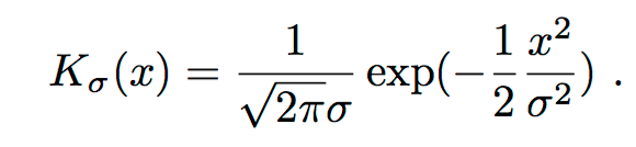
Figure : Gaussian Kernel used for Kernel Code book smoothing of the distances between SIFT descriptors and vocabulary.
In this project we use the gaussian kernel, which has one free parameter i.e. standard deviation (denoted by sigma). In the figure below, we have shown the different accuracies obtained using kernel codebook encoding.
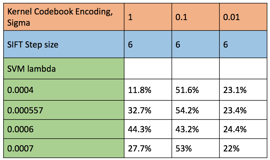
Figure : Accuracy of various combination of parameters for kernel codebook encoding of SIFT descriptors and classification using SVM.
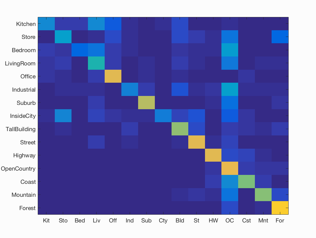
Figure : Confusion matrix for best consistent accuracy = 54.2%% obtained using Kernel standard deviation sigma = 0.1, sift step size = 6, and SVM lambda = 0.000557.
Analysis of results for Kernel Codebook Encoding:
Using this image representation technique, we again switch gears slightly. Here kernel encoding requires a gaussian kernel. The free parameters in this is the variance of gaussian kernel. As we kernelize SIFT features, we have the free parameters of SIFT as well. We continue to use SVM classifier, which gives us regularization parameter to be tuned.
- For SIFT, we maintain the SIFT step size of 6, as we observed that gives us consistent results.
- The next free parameter is the standard deviation of gaussian kernel. We try a range of variables from 100 to 0.01. The only significant results were obtained using sigma = 0.1. This is because, the the other gaussians are too selective with low variance, or too large for the images in the given train and dataset. This sigma of 0.1 is a sweet spot.
- The next free parameter is the regularization parameter of SVM classifier. Here we try a number of values ranging from 10 to 0.0001. We find comparable accuracies for lambda = 0.00043 and 0.000557. Higher the lambda, each miss-classification costs too much thus resulting in more false negatives. On the other hand, lower lambda results in too much lax towards miss-classifications thus resulting in more false positives.
- We observe a slight decrease in accuracy from vanilla SIFT to kernel codebook encoding. This is because two features that are close by in euclidean space, may be living in different gaussians. This results in some loss of spatial correlation during the encoding process. As the SVM is done in euclidean space, and considers euclidean distance, two features that are supposed to be close by are pushed away from each other, thus increasing the chance of miss-classification.
VIII. Combination of SIFT, GIST, Fisher encoding and Spatial pyramid.
In an attempt to understand the behaviour of the various techniques, we execute one test case with all the image representations combined. As all the features are of different width, we horizontally concatenate them to have a long vector representation for each image. We use three levels of spatial encoding as done in section 4. We observe that the results are uncannily similar to those of only Fisher encoding. To understand this, we observe the feature vector itself of each image. We notice that Fisher vector length is about 7000 (depending on number of GMM clusters). Thus a major chunk of infomation in each vector is provided by fisher encoding, whereas the SIFT and GIST add a negligible 400 dimensions. This is possibly the reason for not observing any change in accuracy on combination of all image representation methods. The table of accuracies is showsn below, with best test case's confusion matrix.
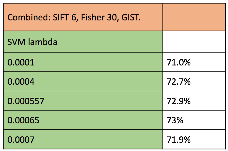
Figure : Accuracy of all combination of image representations, with classification using SVM.
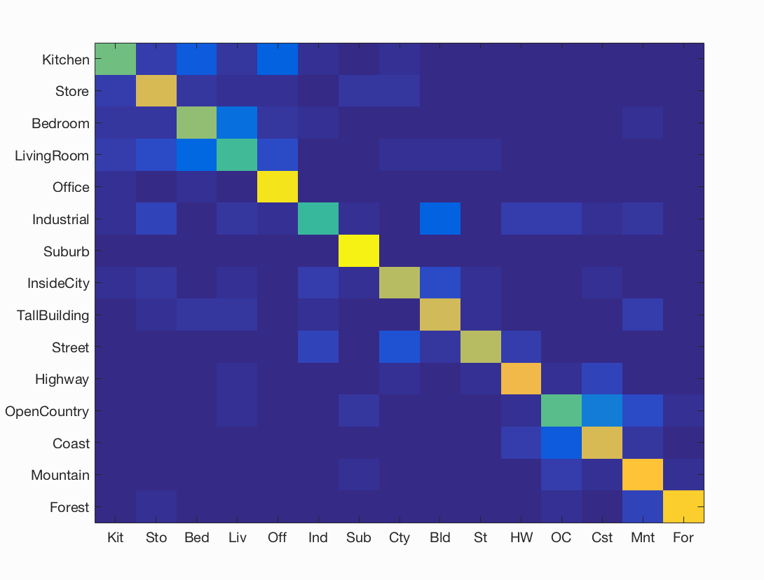
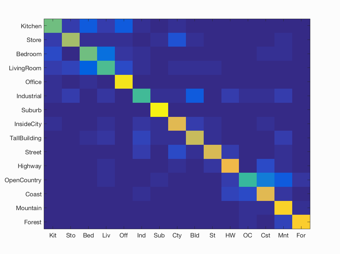
Figure : Confusion matrix for best consistent accuracy = 72.9%% obtained using Fisher encoding of GMM clusters =30, sift step size = 6, and SVM lambda = 0.000557.
Results visualization for best performing recognition pipeline
Combination: Fisher Encoding (GMM cluster size 30, SIFT step size 6) with Linear SVM Classification (lambda = 0.000557).
Accuracy (mean of diagonal of confusion matrix) is 0.592
| Category name | Accuracy | Sample training images | Sample true positives | False positives with true label | False negatives with wrong predicted label | ||||
|---|---|---|---|---|---|---|---|---|---|
| Kitchen | 0.620 |  |
 |
 |
 |
 Bedroom |
 Bedroom |
 Industrial |
 Bedroom |
| Store | 0.500 | 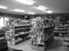 |
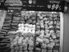 |
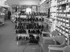 |
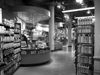 |
 LivingRoom |
 InsideCity |
 Bedroom |
 Bedroom |
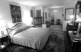
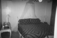
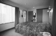
| Bedroom | 0.380 | 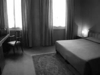 |
 |
 |
 |
 Kitchen |
 Industrial |
 LivingRoom |
 Coast |
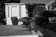
| LivingRoom | 0.310 |  |
 |
 |
 |
 Bedroom |
 Industrial |
 Bedroom |
 Suburb |
| Office | 0.700 |  |
 |
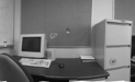 |
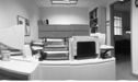 |
 Kitchen |
 Store |
 Kitchen |
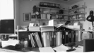 InsideCity |
| Industrial | 0.270 |  |
 |
 |
 |
 InsideCity |
 Store |
 TallBuilding |
 Kitchen |
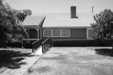
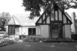
| Suburb | 0.810 |  |
 |
 |
 |
 Highway |
 OpenCountry |
 LivingRoom |
 Store |
| InsideCity | 0.400 |  |
 |
 |
 |
 Suburb |
 TallBuilding |
 Street |
 LivingRoom |
| TallBuilding | 0.740 |  |
 |
 |
 |
 OpenCountry |
 Bedroom |
 Coast |
 Mountain |
| Street | 0.700 |  |
 |
 |
 |
 Forest |
 Industrial |
 Industrial |
 InsideCity |
| Highway | 0.710 |  |
 |
 |
 |
 Industrial |
 Industrial |
 Office |
 LivingRoom |
| OpenCountry | 0.480 |  |
 |
 |
 |
 Industrial |
 Highway |
 Suburb |
 Coast |
| Coast | 0.700 |  |
 |
 |
 |
 Industrial |
 OpenCountry |
 Highway |
 Suburb |
| Mountain | 0.680 |  |
 |
 |
 |
 Industrial |
 Store |
 Suburb |
 Street |
| Forest | 0.880 |  |
 |
 |
 |
 OpenCountry |
 OpenCountry |
 OpenCountry |
 Suburb |
| Category name | Accuracy | Sample training images | Sample true positives | False positives with true label | False negatives with wrong predicted label | ||||
Lorem ipsum dolor sit amet, consectetur adipisicing elit, sed do eiusmod tempor incididunt ut labore et dolore magna aliqua. Ut enim ad minim veniam, quis nostrud exercitation ullamco laboris nisi ut aliquip ex ea commodo consequat. Duis aute irure dolor in reprehenderit in voluptate velit esse cillum dolore eu fugiat nulla pariatur. Excepteur sint occaecat cupidatat non proident, sunt in culpa qui officia deserunt mollit anim id est laborum.