Project 4 / Scene Recognition with Bag of Words
This project includes the task of scene recognition using nearest neighbor and linear SVM classification techniques on bags of quantized local features (SIFT).
The sections of the report are as follows:
- Tiny images with Nearest neighbor classification
- Bag of Words with Nearest neighbor classification
- Bag of Words with linear SVM classification
- Extra Credits
- Results
- Conclusion
Tiny images with Nearest neighbor classification
In this, images are resized to 16X16 and are made zero mean and unit length before using NN classification. The table below presents the results with different numbers of neighbors. The best accuracy (23.4%) can be observed for N=11.
| Nearby Neighbors(Knn) | Accuracy % |
| 1 | 22.5 |
| 5 | 22.3 |
| 7 | 23.1 |
| 11 | 23.4 |
| 21 | 22.6 |
Bag of Words with Nearest neighbor classification
The model ignores or downplays word arrangement and classifies based on a histogram of the frequency of visual words. The vocabulary is established by the local features (SIFT Features). For the experiments, vlfeat library package is used. This technique consists of three parts:
- Build Vocabulary of local features using k-means (Parameter: vocab size, step size)
- Get bags of SIFT features for train and test images (Parameters: step size )
- Classify test images using some metric (Parameters: number of nearest neighbors, SVM - Lambda)
The results below are presented for step size = 3, vocabulary size = 200 with KNN classification algorithm. The best accuracy (55.3%) can be observed for N=5.
| Nearby Neighbors(Knn) | Accuracy % |
| 1 | 54.3 |
| 5 | 55.3 |
| 7 | 54.0 |
| 11 | 54.1 |
| 21 | 52.7 |
Bag of Words with linear SVM classification
The same steps are followed as mentioned above. Only the classifier used is linear SVM. The basic version with step size = 8, gives accuracy = 66.9%. The results below are presented for step size = 3, vocabulary size = 200 with linear SVM classification algorithm for different Lambda. The best accuracy (71.7%) can be observed for Lambda=0.00011 (The tuned version in the code).
| SVM Lamba | Accuracy % |
| 1 | 34.7 |
| 0.01 | 54.9 |
| 0.001 | 62.9 |
| 0.00011 | 71.7 |
| 0.00001 | 67.7 |
| 0.000001 | 62.9 |
Extra Credits
1. Different Vocabulary Sizes and Performance Impact
For the experiments, as I needed to run the recognition steps from the beginning (vocabulary building step) for different vocabulary sizes, I changed the step size to 8 from 3, as 3 was consuming a lot of time to produce the results. With this new step size, I could still observe the trend on changing the step-size which is the intent of this exercize. I have added a table entry that just shows the time consumed specifically by k-means algorithm while building the vocabulary
| Vocabulary Size | Accuracy KNN % | Accuracy Linear SVM % | Time by K-means (sec) |
| 10 | 41.7 | 41.2 | 9.02 |
| 20 | 47.6 | 50.76 | 23.9 |
| 50 | 53.1 | 61.1 | 56.32 |
| 100 | 54.4 | 63.5 | 99.11 |
| 200 | 55.1 | 66.3 | 257.28 |
| 400 | 56.7 | 67.7 | 618.68 |
| 1000 | 55.7 | 69.5 | 1465.21 |
From the table above, it can be seen that on increasing the vocabulary size, the accuracy improves because of more centroids and better classification. But, it impacts the performance significantly. The iteration with size = 1000, took huge amount of time for little accuracy gain over step size = 400. So, its a trade-off between performance and accuracy.
2. SVM with chi-square Kernel
Used SVM with chi-square kernel from the VLfeat library package. The features are represented in higher dimensions (it increased to 1000 from 200) to find better hyperplane to separate the input data. The time for running the recognition task got increased because of the higher dimensionality of the features. I could see the improvement over the linear SVM for a given Lambda.Step size used is 3. The best accuracy (73.2%) can be observed for Lambda=0.0003.
| Kernal | Lambda | Accuracy % |
| Linear | 0.00011 | 71.7 |
| Chi Square | 0.00011 | 70.1 |
| Chi Square | 0.0002 | 71.8 |
| Chi Square | 0.0003 | 73.2 |
3. Kernal Codebook Encoding
Instead of adding 1 to the bin for the feature closest to one of the cluster, it is suggested that contribution of feature should be observed by all the bins based on its distance from the bins (inversaly proportional to the distance). As proposed in paper, descriptors are assigned in a soft manner. weightedBin = exp(-d^2/2 * v) here d is the the distance and v is taken as 8000. I ran this test for step size = 8, to avoid long runs. But on comparing it with values in section-1 of Extra Credits of different vocabulary sizes, the accuracy comes out to be 59.5 % for SVM's Lambda = 0.000001 (This Lambda was giving the best result) which is less that than the value specified above (66.5) and for Knn (n=11) it is 43.2%.
One of the online sources mentioned to use distance metric of k-nearest neighbor (I took k = 11) and added their inverse weighted distance to histogram bins with the same formula as mentioned above. Its different from the previous implementation, as only a subset of features provide their contributions. I kept step size of 8 to get better performace. I didn't see any improvement with this as well. Liner SVM with Lambda=0.000001 (This Lambda was giving the best result) is 59.3 % which is very close to result above and for Knn (n = 11) it is 43.3%. Performance wise this implementation would be better.
I assume it might get better by changing "v" values in the formula mentioned and also the smaller step size might have given better results.
4. Fisher Encoding
This encoding captures the average first and second order differences between the image descriptors and the centres of a GMM, which can be thought of as a soft visual vocabulary. I used step size of 8 to increase the speed, took 50 GMM clusters. With this, the number of bins obtained is 2*50*128 = 12800. To implement this, I used vl_gmm and vl_fisher from vlFeat package library. For linear SVM, I could achieve an accuracy of 74.4% for Lambda = 0.00011 which is better than the result of base version and its performance is much better. With chi-square kernel SVM, I could obtain the accuracy of 77.7% with Lambda = 0.0003.
5. Spatial Pyramid
As described in Lecture notes and in paper by Lazebnik et al 2006, I added spatial information to the image features which gave significant improvement in the results. Two Levels were added to basic version. So if the initial vocabulary size = 200, now the total number of bins were 200 (Level 0) + 4 * 200 (Level 1) + 16 * 200 (Level 2). The image features calculation took a significant amount of time due 21 fold increase in the number of bins.
I got an accuracy of 79% on SVM with chi-square kernel for Lambda = 0.0003 (These results are shown below as well for reference) and step size = 3. I tried with several Lambda values but this one gave the best results. With Knn (n = 11), I could get an accuracy of 57.3 % which is the highest for Knn claassification.
My results for linear SVM classifier didn't improve with spatial pyramid. I even lost some accuracy with it. With Lambda = 0.000001, accuracy was 65.2%. I tried with different Lamda but this is the best that I was getting.
6. Features at Multiple Scales
For this, I used impyramid command of Matlab to downsize the image and compute the features again. With these addition, feature calculation time increased significantly, as the number of SIFT features were around 13K, i.e. approximately double the number of features that I used for original image. I used the step size = 3. For Linear SVM, accuracy = 71.3% for Lambda = 0.00011. SVM with chi-square kernel was 72.0% for Lambda = 0.0003 and KNN with n = 11 gave an accuracy = 54.1%
Observation: The results were similar to non scaling version and didnt change significantly, but the compute time increased alot. Probabably selecting a set of SIFT features and tuning Lambda would give better results or overfitting might be happening.
7. Cross Validation
To perform cross validation, I ran 10 iterations to get image features. For each iteration, I used 200 random images from the training set and 100 random images test images to test the accuracy. I used the step size =8 to increase the run speed. The results are not as good as obtained for the complete set of images as expected because of smaller set. Also, test images might be from completely different categories when compared to the randomly selelcted training set. The results are shown below for Linear SVM:
| Iteration | 1 | 2 | 3 | 4 | 5 | 6 | 7 | 8 | 9 | 10 |
| Accuracy % | 53 | 45 | 66 | 53 | 51 | 54 | 57 | 55 | 53 | 53 |
| Average Accuracy | Standard Deviation |
| 54 | 5.25 |
Results with Confusion Matrix
I got the best accuracy of 79% for bag of words with spatial pyramids and chi-square kernel SVM classifier. Lambda = 0.0003, step size = 3, initial vocab_size = 200, total bins = 21 x vocab_size.
Scene classification results visualization
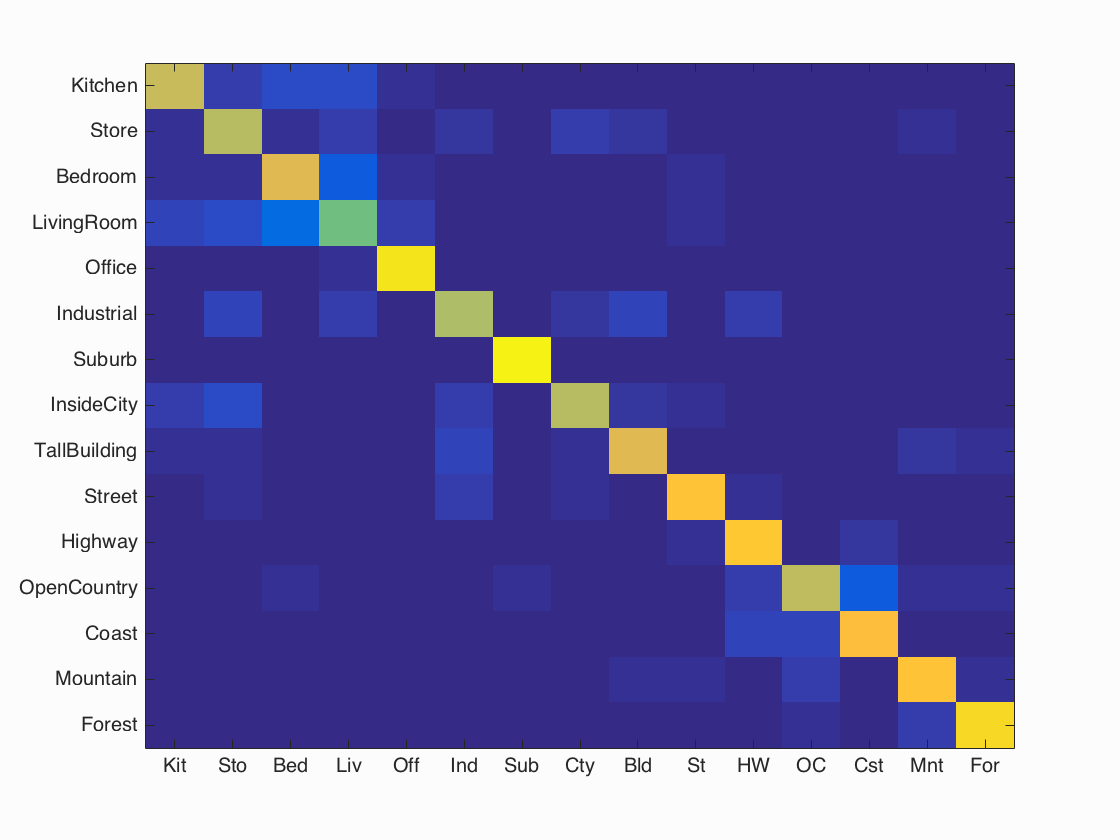
Accuracy (mean of diagonal of confusion matrix) is 0.790
| Category name | Accuracy | Sample training images | Sample true positives | False positives with true label | False negatives with wrong predicted label | ||||
|---|---|---|---|---|---|---|---|---|---|
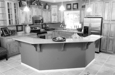
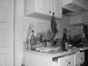
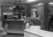
| Kitchen | 0.720 | 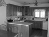 |
 |
 |
 |
 InsideCity |
 TallBuilding |
 Store |
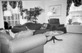
 LivingRoom |
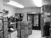
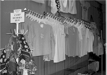
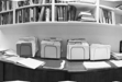
| Store | 0.690 | 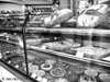 |
 |
 |
 |
 InsideCity |
 LivingRoom |
 TallBuilding |
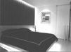
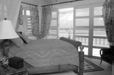
 Bedroom |
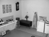
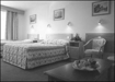
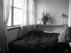
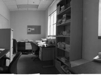
| Bedroom | 0.770 | 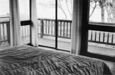 |
 |
 |
 |
 LivingRoom |
Store |
 Office |
 LivingRoom |
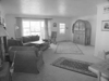
| LivingRoom | 0.580 | 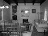 |
 |
 |
 |
 Kitchen |
 Store |
 Store |
 Bedroom |
| Office | 0.950 |  |
 |
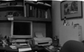 |
 |
 Kitchen |
 Mountain |
 Bedroom |
 LivingRoom |
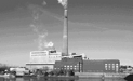
| Industrial | 0.680 | 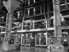 |
 |
 |
 |
 Street |
 InsideCity |
 Store |
 InsideCity |
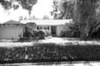
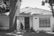
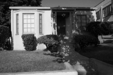
| Suburb | 0.970 | 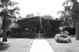 |
 |
 |
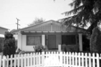 |
 OpenCountry |
 Forest |
 InsideCity |
 LivingRoom |
| InsideCity | 0.690 |  |
 |
 |
 |
 Store |
Suburb |
 Kitchen |
 Store |
| TallBuilding | 0.770 |  |
 |
 |
 |
Industrial |
 Mountain |
 Industrial |
 Coast |
| Street | 0.850 |  |
 |
 |
 |
 Highway |
 Mountain |
 Industrial |
 Industrial |
| Highway | 0.870 |  |
 |
 |
 |
 Coast |
 Coast |
 Coast |
 Bedroom |
| OpenCountry | 0.710 |  |
 |
 |
 |
 Street |
 Forest |
 Suburb |
 Bedroom |
| Coast | 0.830 |  |
 |
 |
 |
 OpenCountry |
 OpenCountry |
 Highway |
| Mountain | 0.850 |  |
 |
 |
 |
 Store |
 OpenCountry |
 TallBuilding |
 Street |
| Forest | 0.920 |  |
 |
 |
 |
 TallBuilding |
 Mountain |
 Mountain |
 OpenCountry |
| Category name | Accuracy | Sample training images | Sample true positives | False positives with true label | False negatives with wrong predicted label | ||||
It can be seen that out of the 15 categories, Living room (accuracy = 58%) gave the least number of true positives, and suburb scenes (accuracy = 97%) gave the maximum true positives.
Conclusion
The project introduced scene recognition. The task was performed on tiny images with nearest neighbors classifier (Accuracy = 23%),on different dataset for bag of words with nearest neighbor (Accuracy = 54.1%) and bag of words with linear SVM (Accuracy = 71.7%). To further improve the accuracy, I got the best results for bag of words with spatial pyramids and chi-square kernel (Accuracy = 79%). It was observed that results vary with different step sizes of dense sift functions. So, increasing step size improves the performance but deteriorates the accuracy. Hence there is trade-off between the accuracy and performance. Changing the vocabulary size (extra credits) affects accuracy as with more bins, better classification is observed till an upper limit. This also impacts the performance alot.For SVM, Lambda parameter impacts the accuracy significantly, so it is tuned for each case separately while reporting the numbers. Adding the spatial information with the SIFT features improved the results significantly with kernal SVM. Different encoding strategies were employed, out of which Fisher gave really good results and good performance. I believe combination of Fisher Encoding + Spatial information + chi-square kernel SVM would give really good results, although it would worsen the performance as the number of bins would increase enormously.