Project 4 / Scene Recognition with Bag of Words
get_tiny_images
Standardize each image to make comparable with the same dimensions.
- For each image path, read the image. To get the image pixels from the string file path.
- Resize each image into a 16 px by 16 px image. So that we have exactly 256 total pixels per image.
- Reshape each image into a single row. So we have a row of 256 values.
- Insert row representing image into the output
image_feats.
nearest_neighbor_classify
Predict the category for every test image by finding the training image with most similar features.
- Get the distances between each pair of training image features and testing image features. So we can use the indices to find the nearest neighbors.
- Get the k-nearest indices for each feature.
- For each k-nearest feature, get the corresponding string label. So we can easily distinguish which is the closest label.
- Get the most common label (from the labels corresponding to the k-nearest features) for each feature. This is the predicted category for that feature.
build_vocabulary
Find cluster centers of SIFT features in vocab_size clusters.
- For each image, get the SIFT features and put them in an array. Use a step of 10 to improve performance.
- Cluster the columns of the matrix of SIFT features in
vocab_sizeclusters. This gets us the cluster centers.
get_bags_of_sifts
Get the normalized frequencies of words per image.
- Get the SIFT features for each image.
- Get the indices of the closest vocab word to each SIFT feature. So we can compare word frequency per image.
- Add up the number of times each index occurs for that image. So we know the frequency of each word per image.
- Divide each index count in each row by the total number of SIFT features found for that image. To normalize the numbers across images so that all frequencies add to 1 per image.
- Return results as
image_feats
svm_classify
Assign labels to each test feature.
- For each category, calculate the weight and the offset from
vl_svmtrainusing the train features and labels. This gives us an SVM equation to separate each category from the others (1:all). - For each test feature, find which equation best defines the category. This will be the equation that gives it the highest value when input into a particular SVM equation.
- Assign the category label of the test feature to be the same as the label that corresponds to the SVM equation.
SVM Lambda
The lambda in vl_svmtrain that gave me the best accuracy was 0.00001.
Pipeline Accuracies
Tiny Images + Nearest Neighbor = 0.189
Bag of SIFT + Nearest Neighbor = 0.546
Bag of SIFT + 1 vs All Linear SVM = 0.653
Scene classification results visualization
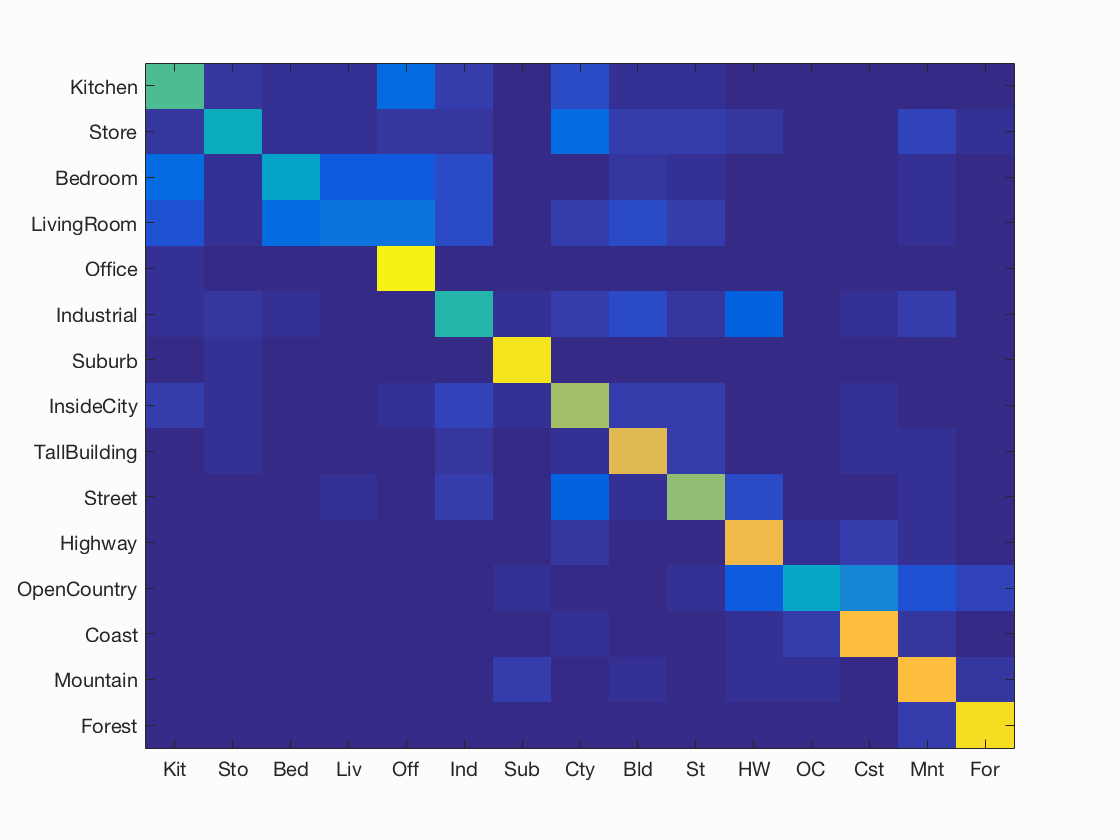
Accuracy (mean of diagonal of confusion matrix) is 0.653
| Category name | Accuracy | Sample training images | Sample true positives | False positives with true label | False negatives with wrong predicted label | ||||
|---|---|---|---|---|---|---|---|---|---|
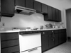
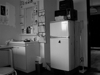
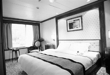
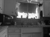
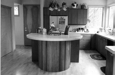
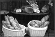
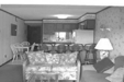
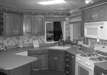
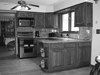
| Kitchen | 0.540 | 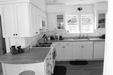 |
 |
 |
 |
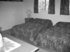
 Bedroom |
 Bedroom |
 InsideCity |
 Office |
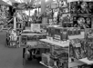
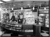
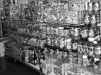
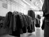
| Store | 0.410 |  |
 |
 |
 |
 TallBuilding |
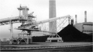
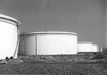
 Industrial |
 TallBuilding |
 Forest |
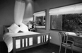
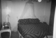
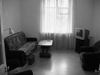
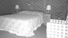
| Bedroom | 0.370 | 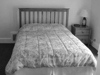 |
 |
 |
 |
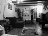
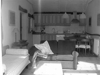 LivingRoom |
 LivingRoom |
 Industrial |
 TallBuilding |
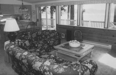
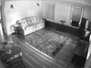
| LivingRoom | 0.190 | 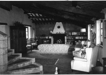 |
 |
 |
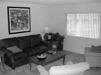 |
 Bedroom |
 InsideCity |
 Office |
 Mountain |
| Office | 0.980 |  |
 |
 |
 |
Kitchen |
 LivingRoom |
 Kitchen |
 Kitchen |
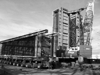
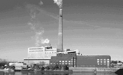
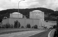
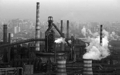
| Industrial | 0.480 | 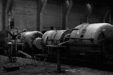 |
 |
 |
 |
 Kitchen |
 Coast |
 InsideCity |
 Highway |
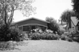
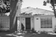
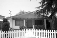
| Suburb | 0.950 | 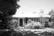 |
 |
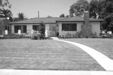 |
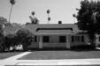 |
 Industrial |
 OpenCountry |
 InsideCity |
 Store |
| InsideCity | 0.660 |  |
 |
 |
 |
 Kitchen |
 Street |
 Industrial |
 Street |
| TallBuilding | 0.770 |  |
 |
 |
 |
Bedroom |
 Store |
 Forest |
 Mountain |
| Street | 0.640 |  |
 |
 |
 |
 Industrial |
 TallBuilding |
 Highway |
 TallBuilding |
| Highway | 0.810 |  |
 |
 |
 |
 Street |
 Coast |
 Coast |
 Coast |
| OpenCountry | 0.390 |  |
 |
 |
 |
 Bedroom |
 Mountain |
Suburb |
 Coast |
| Coast | 0.830 |  |
 |
 |
 |
 OpenCountry |
 OpenCountry |
 InsideCity |
 Highway |
| Mountain | 0.840 |  |
 |
 |
 |
 Industrial |
 Street |
 OpenCountry |
 Suburb |
| Forest | 0.930 |  |
 |
 |
 |
 OpenCountry |
TallBuilding |
 Mountain |
 Mountain |
| Category name | Accuracy | Sample training images | Sample true positives | False positives with true label | False negatives with wrong predicted label | ||||