Project 4 / Scene Recognition with Bag of Words

Tiny Image + Nearest Neighbor Classifier

For the Tiny Image features, we simply resize each image to 16x16 and reshape it to a vector of 256.
In the nearest neighbor classifier, we use vl_alldist2 to calculate the distances. Thereafter we sort each row using the sort function. We then pick the most frequent label among the nearest k neighbors.
I found that k = 1 to be an appropriate value for this case. This gives an accuracy of 0.19 whereas k = 25 gives an accuracy of 0.185, which is not too different. (Specifically k=25 because that is the tuned value that we use for bag of SIFT).
This condition runs in close to 11 seconds

Bag of SIFT + Nearest Neighbor Classifier

In the build_vocabulary function, we use a step size of 32, and a bin size ('size' parameter) of 16. This seemed to provide better overall accuracy. Previously I was using the fast parameter here and a smaller bin size. It is justified to not use the fast parameter while computing the vocabulary because this is computed only once.
In the get_bags_of_sifts function, we use a step size of 8, a bin size of 16 and the fast parameter. I experimented with different step sizes, with 4 the runtime came to more than 10 minutes (without vocabulary building) and at higher values, the accuracy was just not enough. We use alldist2 to calculate the distance between each sift vector in the image with the vocabulary. We hence compute the histogram of the sift features for this image. Ultimately, we normalize the histogram so that number of features found in an image doesn't tamper with the results. The normalization also helped improve the accuracy of the condition.
As stated above, we use a k=25 value for the nearest neighbor classifier.
The accuracy we find in this condition is: 0.515 with a run time of 193 seconds (just over 3 minutes).

Bag of SIFT + 1-vs-all SVM Classifier

In the SVM classifier, for each category, we generate the binary labels and train the svm for these labels. We store the obtained W and B. Thereafter, for each test data point, we compute the confidence for each of the svms and consequently predict the label based on the highest confidence value.
For the regularization parameter, I found that a value of 0.0017 was most appropriate. I tried various values.
The accuracy we find in this condition is: 0.585 with a run time of 191 seconds (just over 3 minutes).

Scene classification results visualization

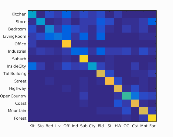
Accuracy (mean of diagonal of confusion matrix) is 0.585

Category name	Accuracy	Sample training images		Sample true positives		False positives with true label		False negatives with wrong predicted label
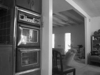
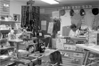
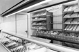
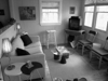
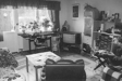
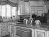
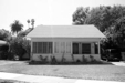
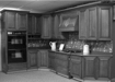
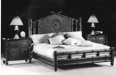
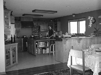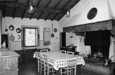
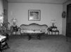
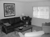
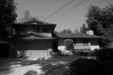
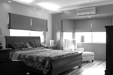
Kitchen	0.370					LivingRoom	Bedroom	Suburb	LivingRoom
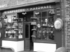
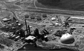
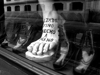
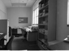
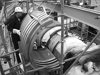
Store	0.340					Industrial	InsideCity	Street	Kitchen
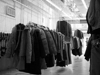
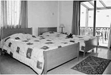
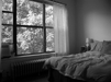
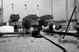
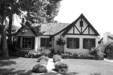
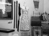
Bedroom	0.280		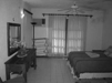			LivingRoom	LivingRoom	Office	Kitchen
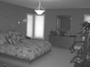
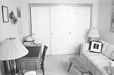
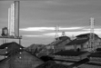
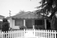
LivingRoom	0.190		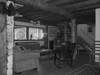			Kitchen	Kitchen	Bedroom	Suburb
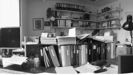
Office	0.870					Bedroom	Kitchen	Kitchen	Kitchen
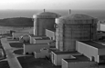
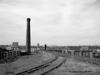
Industrial	0.150		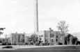			LivingRoom	Kitchen	Mountain	Kitchen
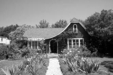
Suburb	0.910					Kitchen	Store	Kitchen	Office
InsideCity	0.350					Kitchen	Kitchen	Industrial	Office
TallBuilding	0.750					Store	Street	Forest	Forest
Street	0.820					InsideCity	InsideCity	Bedroom	Highway
Highway	0.770					Coast	Industrial	OpenCountry	OpenCountry
OpenCountry	0.510					Coast	Highway	Suburb	Highway
Coast	0.790					Bedroom	Store	Highway	OpenCountry
Mountain	0.760					Store	Industrial	OpenCountry	OpenCountry
Forest	0.910					Store	Industrial	Mountain	Mountain
Category name	Accuracy	Sample training images		Sample true positives		False positives with true label		False negatives with wrong predicted label