Project 4 / Scene Recognition with Bag of Words
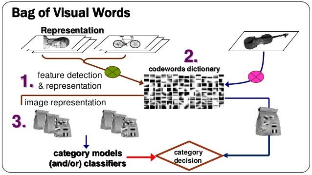
Example of bag of words using visual dictionary pipeline.
The aim of this project was to understand about the basic bag of words pipeline and about the image/scene recognition. The image features were represented using the downsampling or tiny images and the SIFT features. Two classification models were implemented: k-nearest neighbor model and the linear SVM (1-vs-all SVMs). Fifteen scenes were given for classification. The pipeline was implemented in the following order :
- Tiny Images and nearest neighbor classifier
- Bag of SIFT representation and nearest neighbor classifier
- Bag of SIFT representation and linear SVM classifier
Image Features Representation
The images were downsampled to the recommended size of 16X16 and were normalized.
The dictionary of visual words was created using the k-means clustering. This dictionary contained the centroids of the clusters. The Scale Invariant Feature Transformation or the features extracted were represented as a histogram. The bin size was used as 8, so as to get the features of dimension 128. One of the parameter which can be varied was the number of features to be retained after implementing vl_dsift. The parameters were changed and the accuracies were measured.
Classifier
The simplest classifier used for classfication. The distance metric is used to calculate the nearest neighbors and after voting the neighbors corresponding to the category the maximum number of times is assigned as the final label.
Support Vector Machine works well and given a line separating the two linearly separated classes. But in this case there were 15 classes to be classified. The technique one vs all was used to get the hyperplane separating all the classes. The SVM was run for the number of classes and the classification was made by using the parameters obtained from all the run.
Results in a table
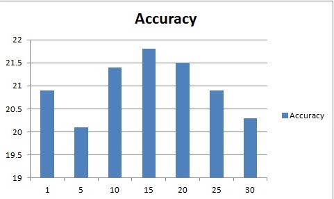
| Value of k used | Accuracy |
|---|---|
| 1 | 20.9 |
| 5 | 20.1 |
| 10 | 21.4 |
| 15 | 21.8 |
| 20 | 21.5 |
| 25 | 20.9 |
| 30 | 20.3 |
Timing Analysis : As the value of k of increased, more time was taken by the program to execute.
|
The x-axis shows the value of k and the y-axis shows the accuracy of classification with respect to the changing value of k. The maximum accuracy was obtasined by using k = 15.
| Cluster Size/Vocab Size | Value of k used | Accuracy | |
|---|---|---|---|
| 10 | 1 | 37.1% | |
| 10 | 15 | 44.9% | |
| 10 | 30 | 46.2% | |
| 50 | 1 | 45% | |
| 50 | 15 | 48.7% | |
| 50 | 30 | 47.1% | |
| 100 | 1 | 51.6% | |
| 100 | 15 | 40.9% | |
| 100 | 30 | 42.3% | |
| 200 | 1 | 50.1% | |
| 200 | 15 | 50.2% | |
| 200 | 30 | 52.0% |
The observation was as the size of cluster size was increased the accuracy became better. At the same time as the value of the nearest neighbor was increased, the accuracy improved. But further increasing the value of the neighbors, decreased the accuracy.
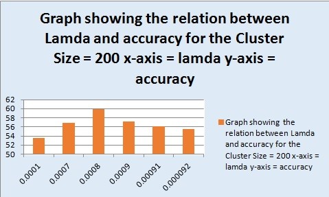
| Cluster Size/Vocab Size | Value of lamda | Accuracy | |
|---|---|---|---|
| 10 | 0.0001 | 45.6% | |
| 10 | 0.001 | 37.9% | |
| 10 | 0.01 | 32.9% | |
| 10 | 1 | 20.1% | |
| 50 | 0.0001 | 53.6% | |
| 50 | 0.001 | 50.1% | |
| 50 | 0.01 | 39.3% | |
| 50 | 1 | 31.3% | |
| 100 | 0.0001 | 59.9% | |
| 100 | 0.001 | 58.6% | |
| 100 | 0.01 | 40.5% | |
| 100 | 1 | 38.0% | |
| 200 | 0.0001 | 53.6% | |
| 200 | 0.0007 | 56.9% | |
| 200 | 0.0008 | 59.9% | |
| 200 | 0.0009 | 57.2% | |
| 200 | 0.00091 | 56.1% | |
| 200 | 0.00092 | 55.5% |
|
The x-axis shows the value of lamda and the y-axis shows the accuracy of classification with respect to the changing value of lamda. The maximum accuracy was obtained by using cluster size = 200 and lamda = 0.0008.
|
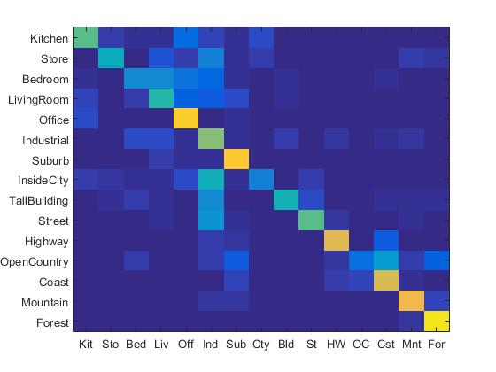
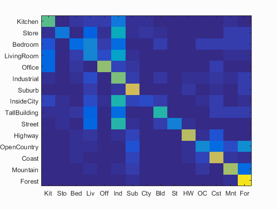
Confusion Matrix for the best result obtained with bag of SIFTs and SVM for the cluster size 200 and the value of lamda = 0.0008.
The SVM's accuracy is very sensitive to the value of lamda.It is very important to choose the correct value of lamda along with the cluser size in order to get the best accuracy. There are a lot of free parameters which can be tuned to get good results. Finally when the results were not satisfactory with the cluster size of 100, for cluster size of 200, a beam search on the values of lamda was done and the values were narrowed down in the range 0.0007-0.001. After getting the range the value of lamda was further tuned to get the final value.
Extra Credit
- Features at multiple scales
- Add complementary features
- Kernel Book Encoding
- Feature Encoding using Fisher Encoding
- SVM with more sophisticated kernels (Kernels used : Chi-squared and RBF kernel)
- Cross-validation to measure performance
- Also, for cross validation and for final fine tuning of the parameters, 100 images from the test data set were kept separately. The pipeline was trained for 1500 training images and was tested on 1400 test images. Once the cluster size was set to 200 and the value of lamda was set to 0.00072, finally the results were run on the 100 separately kept images.
- Experimentation with different vocabulary size
For the baseline, the features were extracted from the images given to us. The results were decent but more the number of features better can be the results. So the features were extracted at multiple scales and the results were run for the scales individually and when all the features from all the scales were combined together. There was a change in the result but not a very drastic change in it.
| Level of the pyramid | Accuracy |
|---|---|
| Level 0 | 59.7% |
| Level 1 | 61.5% |
| Level 2 | 58.8% |
|
The confusion Matrix showing the results obtained by combining the fatures of the original image with the first level downsampled image. The accuracy obtained was 61.5%
GIST features were added to the SIFT features before sending the features to the classifier. The gist_descriptors were calculated using LMgist function. This functiona normalizes the features, so separate normalization is not required. This improved the accuracy of categorization. The cluster size was considered to be 200.
k-nearest neighbour
| Value of the neighbors (k) considered | Accuracy |
|---|---|
| 1 | 61.1% |
| 15 | 62.4% |
| 30 | 62.7% |
SVM classifier
| Value of Lamda | Accuracy |
|---|---|
| 0.0009 | 68.6% |
| 0.001 | 69.8% |
| 0.002 | 69.5% |
| 0.003 | 66.9% |
This is the technique of allowing a degree of flexibility while assigning the visual features to a single codeword as opposed to the hard assignment. This soft assignment technique improves the accuracy while categorizing the datasets. In this technique, the distance of each feature to all the centroids was computed and the weights were assigned to according to the distance to the centroid (lesser the distance more the weight and vice-versa) and finally the sum over all number of the descriptors was taken to create the histogram. Although I expected the accuracy to increase with this encoding but surprisingly it reduced. The categorization accuracy achieved with SVM and vocab size of 200 and lamda 0.0007 was 48.5%. For 100 clusters it came down to 48.0%.
The features can be encoded using more sophisticated feature encoding techniques. The vocabulary was built using the GMM and then the features were extracted using the Fisher Encoding. The results were drastically improved using this.
| Value of Lamda | Accuracy with Fisher Encoding | Accuracy with Fisher Encoding and Chi-Squared Kernel for SVM |
|---|---|---|
| 0.00072 | 73.3% | 77.9% |
| 0.00075 | 73.5% | 77.2% |
| 0.0009 | 73.1% | 77.7% |
Using more sophisticated kernel meant the improvement in the accuracy, but the results did not improve drastically.
The following table presents the results using the Chi-squared kernel.
| Value of Lamda | Accuracy without including the GIST descriptors | Accuracy with including the GIST descriptors |
|---|---|---|
| 0.0004 | 50.30% | 59.10% |
| 0.0005 | 48.30% | 63.50% |
| 0.0007 | 48.70% | 63.33% |
| 0.0009 | 53.20% | 63.10% |
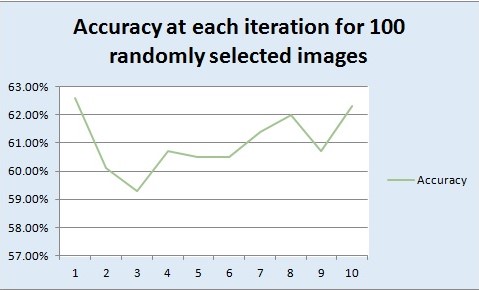
Randomly picked up 100 images from the training dataset and 100 images from the testing dataset. For a step size of 8 and vocab size of 200, extracted the features and measured the accuracy of categorization for 10 different iterations, each time randomly 100 different images were picked up. Finally, the average and the standard deviation of the performance was measured. This was run for a step size of 8 for extracting the features and the the value of lamda used for SVM classifier was 0.00072.
| No of iterations | Accuracy |
|---|---|
| 1 | 62.6% |
| 2 | 60.10% |
| 3 | 59.30% |
| 4 | 60.70% |
| 5 | 60.50% |
| 6 | 60.50% |
| 7 | 61.40% |
| 8 | 62.0% |
| 9 | 60.70% |
| 10 | 62.30% |
|
The x-axis shows the number of iterations and the y-axis shows the accuracy of categorization. The average performance reported was 61.01% and the standard deviation achieved was 0.0104. From the accuracy we can see the variation because at different time different images will be picked up. Sometimes some features of a particular category can be seen while others will be missed. So we get random accuracies everytime.
The vocabulary size of 10, 50, 100 and 200 was used to check the results. The results are reported above with the normal pipeline.
Scene classification results visualization
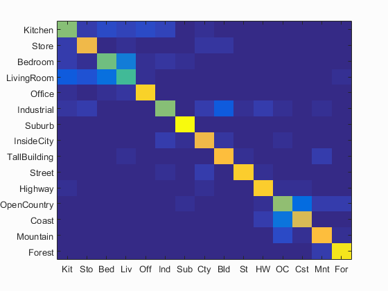
Accuracy (mean of diagonal of confusion matrix) is 0.776
| Category name | Accuracy | Sample training images | Sample true positives | False positives with true label | False negatives with wrong predicted label | ||||
|---|---|---|---|---|---|---|---|---|---|
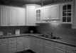
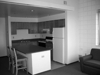
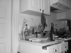
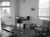
| Kitchen | 0.610 | 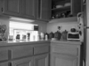 |
 |
 |
 |
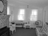
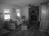
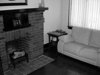
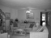 LivingRoom |
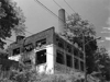
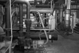
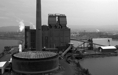 Industrial |
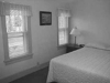
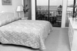
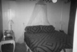
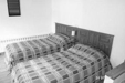
 Bedroom |
 Bedroom |
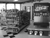
| Store | 0.810 | 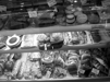 |
 |
 |
 |
 LivingRoom |
 LivingRoom |
 LivingRoom |
 InsideCity |
| Bedroom | 0.580 |  |
 |
 |
 |
 LivingRoom |
 TallBuilding |
 Industrial |
 LivingRoom |
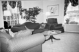
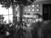
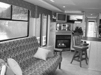
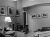
| LivingRoom | 0.530 |  |
 |
 |
 |
 Bedroom |
 Bedroom |
 Bedroom |
 Kitchen |
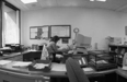
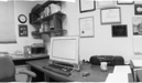
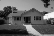
| Office | 0.900 | 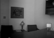 |
 |
 |
 |
 LivingRoom |
 Industrial |
 Kitchen |
 LivingRoom |
| Industrial | 0.620 |  |
 |
 |
 |
 InsideCity |
 Coast |
 TallBuilding |
 Mountain |
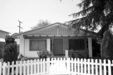
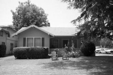
| Suburb | 1.000 | 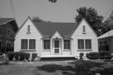 |
 |
 |
 |
 InsideCity |
 OpenCountry |
||
| InsideCity | 0.810 |  |
 |
 |
 |
 Industrial |
Store |
Suburb |
 Store |
| TallBuilding | 0.830 |  |
 |
 |
 |
Industrial |
 Store |
 LivingRoom |
 Mountain |
| Street | 0.880 |  |
 |
 |
 |
 InsideCity |
 Mountain |
 InsideCity |
 Industrial |
| Highway | 0.890 |  |
 |
 |
 |
 Industrial |
 Coast |
 Kitchen |
 Coast |
| OpenCountry | 0.640 |  |
 |
 |
 |
 Coast |
 Coast |
 Forest |
 Mountain |
| Coast | 0.750 |  |
 |
 |
 |
 OpenCountry |
 TallBuilding |
 OpenCountry |
| Mountain | 0.840 |  |
 |
 |
 |
 OpenCountry |
TallBuilding |
 OpenCountry |
 Coast |
| Forest | 0.950 |  |
 |
 |
 |
 Mountain |
 OpenCountry |
 Mountain |
 Mountain |
| Category name | Accuracy | Sample training images | Sample true positives | False positives with true label | False negatives with wrong predicted label | ||||