Project 4 / Scene Recognition with Bag of Words
In this project I have experimented with image recognition. I have written and anlyzed few different algorithms in this area that goes from simple methods like tiny images and nearest neighbor classification to more advanced methods like bags of quantized local features and linear classifiers learned by support vector machines. This report is divided in four parts:
- Tiny images representation and nearest neighbor classifier
- Bag of SIFT representation and nearest neighbor classifier
- Bag of SIFT representation and linear SVM classifier
- Extra Credits
Let's go through each of them:
1. Tiny images representation and nearest neighbor classifier
- Here I 'm first simply resizing each image to a small, fixed resolution 16 x 16. Then I transform this image such that it has zero mean and unit length. Because it discards all of the high frequency image content and is not especially invariant to spatial or brightness shifts, it is not really a good represntation.
- Then I 'm using K-nearest neighbour method for classification. It has many desirable features like it requires no training, it can learn arbitrarily complex decision boundaries, and it trivially supports multiclass problems etc.
- To tackle its disadvantage of being quite vulnerable to training noise, I have implemented voting based on the K nearest neighbors, a more general form of 1-NN.
- Here are the results I obtained in my experiment:
K Accuracy(%) 1 22.5 3 21.5 5 21.3 7 21.1 9 21.1 11 21.8 13 22.3 15 22.5 - As we can see from the results, with tiny images as the features, varying K didn't really had any significant effect on the accuracy with test data set.
2. Bag of SIFT representation and nearest neighbor classifier
- Here I 'm first building a vocabulary of visual word. I sample many local SIFT features from the training set (15000 - 1600000). I choose a specific number of clusters and then cluster them with K-means. The number of clusters is my vocab size
- . Now our feature representation of the images are histograms of these visual words. I obtain this histogram by simply counting number of SIFT descriptor falling into each cluster of my vocabulary. Also I 'm normalizing these histograms to remove the effect of feature magnitude.
- I run K-nearest neighbour now on these features for classification. I have played with 4 parameters from K-NN to SIFT to tune:
- Here are the results I obtained in my experiment:
Vocab Size = 100, Features per image = 100, Step size = 4 K Accuracy(%) 1 50.4 3 50.3 5 51.9 7 51.8 9 51.6 11 50.6 15 50
Vocab Size = 100, Features per image = 100, Step size = 8 K Accuracy(%) 1 48.1 3 49.1 5 51.1 7 51.7 9 51.9 11 51.2 15 50.9
Vocab Size = 100, Features per image = 100, Step size = 16 K Accuracy(%) 1 43.7 3 43.1 5 44.3 7 44.4 9 43.2 11 43.8 15 43.7 - As we can see from the results, with bag of sifts as the features, varying K improved the accuracy on the test set, probably accounting to better denoising with higher K. The optimum K came to be around 7.
| Parameter | Description |
|---|---|
| Step size | Higher this is is more densely we are sampling SIFT descriptors |
| Features per image | Number of samples randomly picked up from SIFT descriptors |
| Vocab size | Number of clusters formed in K-means |
| K | Number of nearest neighbors in KNN |
3. Bag of SIFT representation and linear SVM classifier
- Here I 'm first building a vocabulary of visual word. I sample many local SIFT features from the training set (15000 - 1600000). I choose a specific number of clusters and then cluster them with K-means. The number of clusters is my vocab size
- . Now our feature representation of the images are histograms of these visual words. I obtain this histogram by simply counting number of SIFT descriptor falling into each cluster of my vocabulary. Also I 'm normalizing these histograms to remove the effect of feature magnitude.
- As this is multi-class classification I have trained 1-vs-all linear SVMS. This method is much better than K-NN not just beacuse of being less expensivep, but because it can learn dimensions of the feature vector that are less relevant and then downweight them when making a decision. I have played with 4 parameters from K-NN to SIFT to tune:
- Here are the results I obtained in my experiment:
Vocab Size = 100, Features per image = 100, Step size = 4 LAMBDA Accuracy(%) 0.00001 61.9 0.0001 62.4 0.001 56.7 0.01 41.9 0.1 43.9 1 30.7 10 37.3
Vocab Size = 100, Features per image = 100, Step size = 8 LAMBDA Accuracy(%) 0.00001 58.3 0.0001 60.3 0.001 54.9 0.01 46.7 0.1 43.9 1 38.2 10 39.1
Vocab Size = 100, Features per image = 100, Step size = 16 LAMBDA Accuracy(%) 0.00001 49.9 0.0001 50.5 0.001 48.2 0.01 41.5 0.1 36.7 1 37.5 10 38.4 - As we can see from the results, with bag of sifts as the features, SVM performed really well comparatively to KNN being less expensive. This shows it less vulneraility to noise in the data. The optimum lambda came to be around 0.0001.
| Parameter | Description |
|---|---|
| Step size | Higher this is is more densely we are sampling SIFT descriptors |
| Features per image | Number of samples randomly picked up from SIFT descriptors |
| Vocab size | Number of clusters formed in K-means |
| LAMBDA | It controls the regularization for the model parameters while learning |
Extra Credits
Experimental design
1. Experiment with different vocabulary sizes
Look for vocab_{size}.mat files in the code directoryI experimented with Bag of SIFT features and SVM learners. From the table we can see that on increasing the vocab size, the performance improved till a certain vocab size after which it started degrading slightly in addition to increased runtime.
| Vocab size | Accuracy(%) |
|---|---|
| 50 | 55.3 |
| 100 | 60.3 |
| 200 | 61.4 |
| 300 | 62.1 |
| 400 | 61.7 |
| 500 | 60.4 |
| 1000 | 59.5 |
2. Cross validation
Code in run_cross_validation.mI ran this 10 times. Each time I took 100 samples per class randomly for both train and test sets. Then ran my baseline mathod of bag of sifts with svm. The result seems to be pretty stable on my final tuned parameters.
| Mean accuracy | 58.39 |
| Standard deviaton | 2.69 |
| Run number | Accuracy(%) |
|---|---|
| 1 | 55.6 |
| 2 | 59.3 |
| 3 | 62.6 |
| 4 | 58.3 |
| 5 | 61.8 |
| 6 | 60.7 |
| 7 | 55.2 |
| 8 | 56.9 |
| 9 | 55.6 |
| 10 | 57.9 |
3. Validation set to tune the model
Code in run_validation_based_tuning.mI experimented with my simple SVM classifier to tune its regularization parameter based on a validation set. I pick my validation set from the training set itself. I 'm doing a 10-fold validation.
Final unused test set accuracy: 60.3| LAMBDA | Mean accuracy(%) | Standard deviation |
|---|---|---|
| 0.000001 | 52.9 | 4.25 |
| 0.00001 | 55.3 | 4.65 |
| 0.0001 | 57.1 | 4.26 |
| 0.001 | 55.7 | 4.05 |
| 0.01 | 41.4 | 3.75 |
| 0.1 | 39.5 | 3.78 |
| 1 | 30.6 | 3.68 |
| 10 | 35.6 | 2.64 |
Feature quantization and bag of words
1. Kernel codebook encoding
Code in get_kernel_codebook.mI have used 'soft assignment' using kernel codebook encoding for bag of words. In this method, assuming a gaussian distribution at each cluster a feature will be assigned to serveral clusters but with a weight that will be proportional to the distance. It performed better than baseline SVM+BOS, but not with significant improved as baseline was 60%. I tried with various sigma and found this as the best value.
Sigma = 210| LAMBDA | Accuracy(%) |
|---|---|
| 10 | 37.3 |
| 1 | 30.7 |
| 0.1 | 43.9 |
| 0.0001 | 49.7 |
| 0.00001 | 59.5 |
| 0.000001 | 64.2 |
| 0.0000001 | 65.3 |
2. Fisher encoding
Code in get_fisher_vectors.mIn addition to keeping the count of descriptors per word, it also encodes additional information about the distribution of the descriptors. As we can see from the results it improved the accuracy significantly from our baseline SVM+BOS which was 60%.
| Number of clusters | Accuracy(%) |
|---|---|
| 10 | 72.0 |
| 10 | 74.3 |
| 50 | 76.1 |
| Number of clusters | Accuracy(%) |
|---|---|
| 10 | 70.3 |
| 30 | 72.1 |
| 50 | 75.3 |
Classifier
1. RBF and Chi-square
Code in get_chisqr_classify.m and get_rbf_classify.mHere, I got good results with Chi-square of around 63.1% but with RBF, the results were not as good, came out to be around 53.2%
Spatial Pyramid representation and classifier
1. Spatial pyramid feature representation
Code in get_spatial_pyramid.mHere I have tried to analyze effects of adding spatial information to the features by creating a grid with varying granularity over the image, therefor making coarser grids. At any fixed level, two points are said to match if they fall into the same cell of the grid. The results are better at higher level as we can see from the results.
| Step size | Pyramid level | Accuracy(%) |
|---|---|---|
| 16 | 0 | 55.1 |
| 16 | 1 | 58.8 |
| 16 | 2 | 62.6 |
| 16 | 3 | 63.9 |
| 8 | 3 | 69.7 |
| 4 | 3 | 70.9 |
Best Result
Although I achieved an accuracy of 76.1 with Step size 4, I would selected step size of 8 for displaying my results as it is easy to reproduce given the time it takes to run. Accuracy = 72.5%, Step size = 8, Fisher
Scene classification results visualization
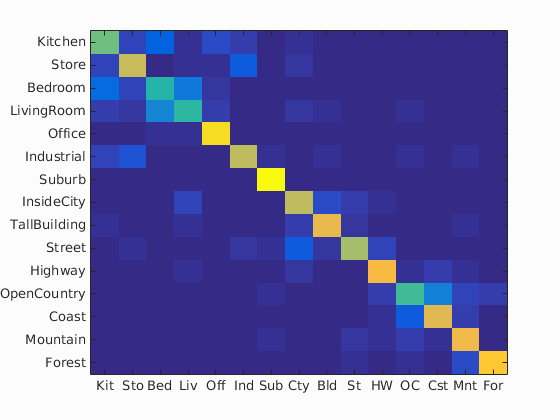
Accuracy (mean of diagonal of confusion matrix) is 0.725
| Category name | Accuracy | Sample training images | Sample true positives | False positives with true label | False negatives with wrong predicted label | ||||
|---|---|---|---|---|---|---|---|---|---|
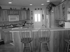
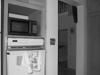
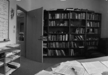
| Kitchen | 0.590 | 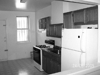 |
 |
 |
 |
 LivingRoom |
 Bedroom |
 Industrial |
 Bedroom |
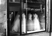
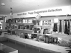
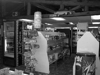
| Store | 0.720 |  |
 |
 |
 |
 LivingRoom |
 Industrial |
 Industrial |
 LivingRoom |
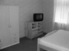
| Bedroom | 0.470 | 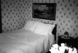 |
 |
 |
 |
 Kitchen |
 LivingRoom |
 Coast |
 Store |
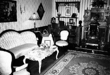
| LivingRoom | 0.490 |  |
 |
 |
 |
 Bedroom |
 Bedroom |
 Store |
| Office | 0.930 |  |
 |
 |
 |
 LivingRoom |
 Kitchen |
 Bedroom |
 LivingRoom |
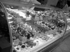
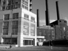
| Industrial | 0.710 | 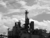 |
 |
 |
 |
 Store |
 Store |
 Store |
 Kitchen |
| Suburb | 0.990 |  |
 |
 |
 |
 OpenCountry |
 InsideCity |
 InsideCity |
|
| InsideCity | 0.710 |  |
 |
 |
 |
 Street |
 Highway |
 TallBuilding |
 Kitchen |
| TallBuilding | 0.790 |  |
 |
 |
 |
 Industrial |
 Street |
 Street |
 Office |
| Street | 0.670 |  |
 |
 |
 |
 InsideCity |
 TallBuilding |
 Industrial |
 InsideCity |
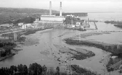
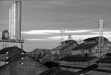
| Highway | 0.820 |  |
 |
 |
 |
 OpenCountry |
 InsideCity |
 InsideCity |
 Coast |
| OpenCountry | 0.530 |  |
 |
 |
 |
 Mountain |
 Coast |
 Coast |
 Coast |
| Coast | 0.780 |  |
 |
 |
 |
 OpenCountry |
 OpenCountry |
 Mountain |
 Mountain |
| Mountain | 0.810 |  |
 |
 |
 |
 Coast |
 Industrial |
 Highway |
 Coast |
| Forest | 0.860 |  |
 |
 |
 |
 TallBuilding |
 OpenCountry |
 Street |
 OpenCountry |
| Category name | Accuracy | Sample training images | Sample true positives | False positives with true label | False negatives with wrong predicted label | ||||