Algorithm Description

Tiny images representation

We simply resize each image to a small, fixed resolution (I took 16x16). This is not a particularly good representation, because it discards all of the high frequency image content and is not especially invariant to spatial or brightness shifts.

Nearest Neighbor Classifier

When classifying a test feature into a particular category, we simply finds the nearest training example using L2 distance as the metric and assign the test case the label of that nearest training example. This is 1-NN. It is quite vulnerable to training noise, though, which can be alleviated by voting based on the K nearest neighbors. We can find the distance from K nearest neighbours and take the mode(most frequently occurring) label among the labels of the k closest neighbours. I implemented both 1-NN,K-NN.

Bag of SIFT representation

We first need to establish a vocabulary of visual words.I used a step size of 5 to create the vocabulary and then clustered them with k-means. I varied the number of clusters and obtained the accuracy for each value of numver of clusters(vocab_size). The centroids of the clusters are stored as vocab.mat. We now represent our training and testing images as histograms of visual words. For each image we will densely sample many SIFT descriptors. Then we count how many SIFT descriptors fall into each cluster in our visual word vocabulary and create corresponding histograms. We normalize the histograms so that image size does not dramatically change the bag of feature magnitude.

Linear SVM Classifier

Linear classifiers are inherently binary and we have a 15-way classification problem. We train 15 binary, 1-vs-all SVMsi.e. each classifier will be trained to recognize 'forest' vs 'nonforest','kitchen' vs 'nonkitchen',etc. Scores are calculated for all 15 classifiers on each test case and the classifier which is most confidently positive "wins".i.e. the one with the highest score.

Extra Credit

Experimental design extra credit:Experimented with many different vocabulary sizes and performance is reported below in RESULTS.

Experimental design extra credit:Randomly pick 100 training and 100 testing images for each iteration, average performance and standard deviations are reported below in RESULTS.

Example of code with highlighting

%example code- get_tiny_images
image=imread(char(image_paths(i)));
image_feats(i,:)=reshape(imresize(image,[16,16]),1,256);

%example code- nearest_neighbor_classify
Distances = vl_alldist2( test_image_feats.',train_image_feats.');
[match, I_match]=sort(Distances,2);
k=1; %taking k nearest neighbours
nearest_neighbours=train_labels(I_match(:,1:k));

%example code- build_vocabulary
[locations, SIFT_ind] = vl_dsift(single(image),'STEP',5,'Fast');

%example code- get_bags_of_sifts
locations, SIFT_feat] = vl_dsift(image,'STEP',10); 
Distances = vl_alldist2(vocab_T,single(SIFT_feat));
[minD,c]=min(Distances);  %c=1Xvocab_size
binranges=1:K;
[histogram]=histc(c,binranges);

%example code- svm_classify
labels1=strcmp(categories(i),train_labels);
labels2(find(labels1))=1;
[W(:,i), B(i)] = vl_svmtrain(single(train_image_feats'), labels2', lambda);

RESULTS

Scene classification results visualization, Vocab_size=200, Step=2 in vl_dsift

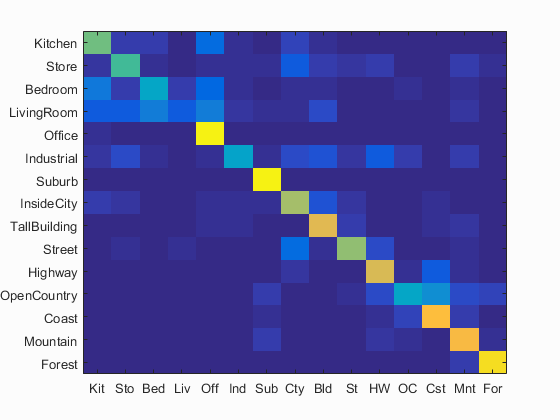
Accuracy (mean of diagonal of confusion matrix) is 0.649

Category name	Accuracy	Sample training images		Sample true positives		False positives with true label		False negatives with wrong predicted label
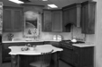
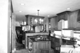
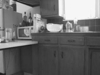
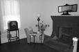
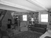
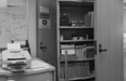
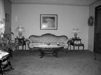
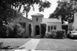
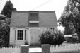
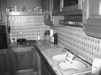
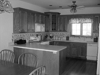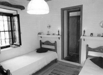
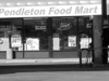
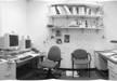
Kitchen	0.590					Bedroom	Store	Office	TallBuilding
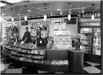
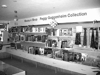
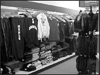
Store	0.520		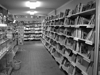			InsideCity	Bedroom	Highway	Mountain
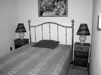
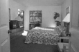
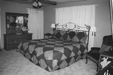
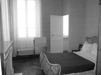
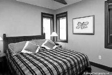
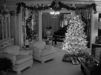
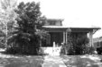
Bedroom	0.390					Industrial	LivingRoom	LivingRoom	Mountain
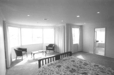
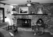
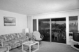
LivingRoom	0.110		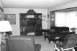			Bedroom	Store	Industrial	Office
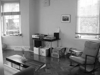
Office	0.970		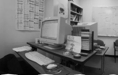			Store	Bedroom	Kitchen	Kitchen
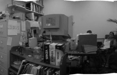
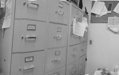
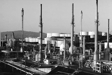
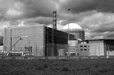
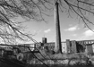
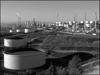
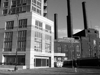
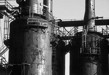
Industrial	0.370					LivingRoom	LivingRoom	Bedroom	Highway
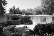
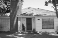
Suburb	0.980		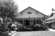			LivingRoom	Mountain	InsideCity	TallBuilding
InsideCity	0.660					Street	Industrial	TallBuilding	Street
TallBuilding	0.780					Industrial	Kitchen	Mountain	Street
Street	0.630					Store	InsideCity	InsideCity	Industrial
Highway	0.760					Street	OpenCountry	Coast	OpenCountry
OpenCountry	0.390					Coast	Coast	Bedroom	Coast
Coast	0.830					OpenCountry	Highway	OpenCountry	Suburb
Mountain	0.820					Store	OpenCountry	Highway	Suburb
Forest	0.930					OpenCountry	OpenCountry	Mountain	Mountain
Category name	Accuracy	Sample training images		Sample true positives		False positives with true label		False negatives with wrong predicted label

RESULTS FOR THE 3 PIPELINES

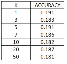
Tiny images representation and nearest neighbor classifier: Accuracy = 0.191 (1-NN)

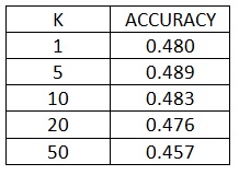
Bag of SIFT representation and nearest neighbor classifier: Accuracy = 0.503 (Step size=3 in vl_dsift, no extra credit)

Bag of SIFT representation and linear SVM classifier: Accuracy = 0.649 (vocab_size=200, Step=2 in vl_dsift)

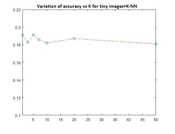
PART 1-Variation of K for K-NN, along with tiny images

The variation of accuracy with respect to k is:

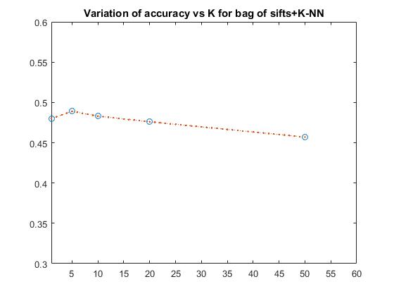
PART 2-Variation of K for K-NN, along with bag of sifts

The variation of accuracy with respect to k is:

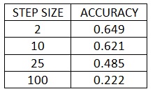
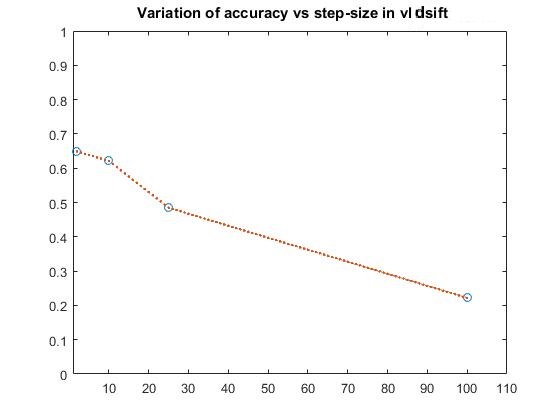
PART 3-Variation of step-size in vl_dsift for bag of sifts+SVM

The variation of accuracy with respect to step-size is:

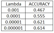
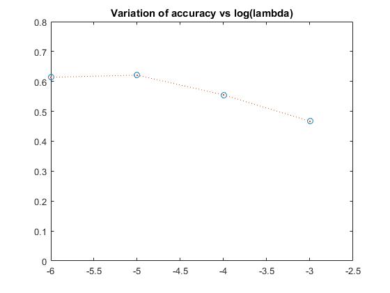
PART 4-Variation of lambda for SVM with bags of sifts

The variation of accuracy with respect to lambda is:

EXTRA CREDIT

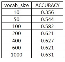
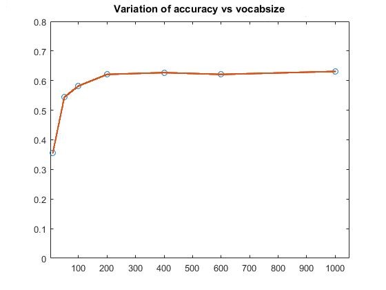
Extra Credit Part 1-Variation of vocab_size

The variation of accuracy with respect to vocab_size is:

Extra Credit Part 2-Taking 100 random training and testing images(over 100 iterations)

The mean of the accuracy is: 0.241

The standard deviation of the accuracy is: 0.135

Since we are taking only 100 training images, the accuracy is lower than that for 1500 training images

Extra Credit Part 3-Add spatial information to your features

I calculated the histograms for each of the 4 quadrants of the image, in addition to 1 histogram of the full original image. The histograms are concatenated together, giving a total number of bins=5 X number of clusters

Step size = 10 in get_bags_of_sifts:

Original accuracy for bags_of_sifts+SVM = 0.621

Accuracy with spatial information included = 0.643(for 4 quadrants of image i.e.2 X 2).

Extra Credit Part 4-Soft assignment of visual words to histogram bins

The weights are calculated as 1/d^2 between each visual word and cluster centre(d=distance). Each visual word now contributes 'weight' value to each histogram bin instead of one for the nearest cluster centre

The accuracy for step size of 10 in get_bags_of_sifts is 0.433.

Since we are taking only 100 training images, the accuracy is lower than that for 1500 training images