Project 4 / Scene Recognition with Bag of Words
For this project, we explored scene recognition strategies via implementations to generate features and to classify based on the features. In particular, there were two feature generation techniques that were implemented: features from tiny images and features generated from a bag of sift features. On the classification front, there were two major implementations in this project: the k-nearest neighbors classifier and the support vector machine (SVM) classifier. We will first go through the implementation of each of these and the impact each has on overall performance, and finally finish with some of the better results that were achieved during this project. The following list below shows the order we will proceed.
- Tiny Image Features
- Nearest Neighbors Classifier
- Bags of SIFT Features
- SVM Classifier
- Building a Vocabulary
- General observations
Tiny Image Features
The idea behind this classifier is that we resize the image inputs to be dxd, where d is some very small power of 2. That's basically it (besides normalizing the numbers in the resized image as well before adding it to the set of features). The instructions suggested 16x16 as a good option, but I chose to test how it worked with other dimensions as well. The numbers will be shown and explained further in the next section where we examine nearest_neighbors.m, but the general trend with tiny_images.m specifically was that both a very small power of 2 and relatively large powers of 2 suffered in terms of accuracy. Finding the proper middle-ground between losing information and retaining information was key to achieving a solid accuracy. Lose too much information and chances are the classifier will overgeneralize to some extent, while if you retain too much, it will likely not generalize enough for its decisions, but it won't necessarily be as bad. For tiny image features in conjunction with the nearest neighbor classifier, a peak accuracy observed was 0.22667 by using 4x4 dimensions for the images and 18 neighbors.
Nearest Neighbor Classifier
For this classifier, we're basically trying to classify using a training image that's most similar in terms of the features of the input image. We have a choice here as to whether we want to look for the nearest neighbor only, or perhaps consider some k number of nearest neighbors when making this decision. In the end, I chose to run this with 20 neighbors, as around that number ended up usually being the ideal amount in terms of peak accuracy. For the table below, it just so happened that k=18 was slightly higher in accuracy, but usually I saw k=20 to be the peak (also, 20 just felt like a nice, perfectly even number to work with). In terms of the nearest neighbor classifier's interaction with the tiny image features, the table below describes the accuracies calculated on runs with a given k number of neighbors and a certain dimension of the tiny image features. As you will see, the global maximum was achieved with 4x4 image features and 18 neighbors, although 20 neighbors was fairly close, and the accuracy gain dampened a lot beyond this point. The row with the most significant difference from the typical results was definitely the 2x2 row. Here you can see we likely lost enough information that even the best classifier would have had a hard time accurately classified the scenes. The larger dimensions performed fairly well too, but definitely not as good as the 4x4 and k=18 or k=20 combination.
| k = 1 | k = 2 | k = 3 | k = 4 | k = 5 | k = 6 | k = 7 | k = 8 | k = 9 | k = 10 | k = 11 | k = 12 | k = 13 | k = 14 | k = 15 | k = 16 | k = 17 | k = 18 | k = 19 | k = 20 | k = 21 | k = 22 | k = 23 | k = 24 | k = 25 | k = 26 | k = 27 | k = 28 | k = 29 | k = 30 | k = 31 | k = 32 | k = 33 | k = 34 | k = 35 | k = 36 | k = 37 | k = 38 | k = 39 | k = 40 | k = 41 | k = 42 | k = 43 | k = 44 | k = 45 | k = 46 | k = 47 | k = 48 | k = 49 | k = 50 | |
|---|---|---|---|---|---|---|---|---|---|---|---|---|---|---|---|---|---|---|---|---|---|---|---|---|---|---|---|---|---|---|---|---|---|---|---|---|---|---|---|---|---|---|---|---|---|---|---|---|---|---|
| 2x2 | 0.08400 | 0.09333 | 0.09867 | 0.09933 | 0.09667 | 0.09733 | 0.09267 | 0.09467 | 0.09733 | 0.10600 | 0.10867 | 0.11000 | 0.10933 | 0.11467 | 0.11133 | 0.11200 | 0.11533 | 0.11533 | 0.10933 | 0.11667 | 0.12200 | 0.12133 | 0.11867 | 0.11267 | 0.11467 | 0.11933 | 0.11467 | 0.12467 | 0.12667 | 0.12333 | 0.12467 | 0.12933 | 0.12600 | 0.12933 | 0.12800 | 0.13133 | 0.13133 | 0.12867 | 0.13333 | 0.12867 | 0.13200 | 0.12800 | 0.13533 | 0.13200 | 0.13200 | 0.12667 | 0.12667 | 0.12533 | 0.12600 | 0.13067 |
| 4x4 | 0.19733 | 0.17333 | 0.18933 | 0.21067 | 0.21933 | 0.22600 | 0.22467 | 0.22067 | 0.22667 | 0.21667 | 0.21533 | 0.21600 | 0.21467 | 0.21733 | 0.22067 | 0.22467 | 0.22400 | 0.22667 | 0.22400 | 0.22600 | 0.22467 | 0.22533 | 0.22467 | 0.22067 | 0.22200 | 0.21667 | 0.22333 | 0.21600 | 0.21600 | 0.21667 | 0.21867 | 0.21733 | 0.21800 | 0.21800 | 0.21733 | 0.21133 | 0.21533 | 0.21400 | 0.21200 | 0.21133 | 0.21067 | 0.21467 | 0.21067 | 0.21200 | 0.21400 | 0.21067 | 0.20733 | 0.20400 | 0.20467 | 0.20600 |
| 8x8 | 0.21733 | 0.18600 | 0.20933 | 0.21000 | 0.21667 | 0.21667 | 0.21667 | 0.21800 | 0.22000 | 0.22000 | 0.21533 | 0.21600 | 0.21867 | 0.21867 | 0.21933 | 0.21867 | 0.22867 | 0.23133 | 0.22733 | 0.22333 | 0.22200 | 0.22333 | 0.22333 | 0.22533 | 0.22733 | 0.22333 | 0.22733 | 0.22533 | 0.22067 | 0.22067 | 0.22267 | 0.22267 | 0.22067 | 0.22467 | 0.22267 | 0.22000 | 0.21933 | 0.21333 | 0.21400 | 0.21467 | 0.21667 | 0.21667 | 0.22133 | 0.22067 | 0.21867 | 0.21733 | 0.21467 | 0.21000 | 0.21333 | 0.21467 |
| 16x16 | 0.22467 | 0.19600 | 0.21867 | 0.20600 | 0.21467 | 0.21400 | 0.21200 | 0.20400 | 0.21333 | 0.21267 | 0.21933 | 0.21600 | 0.22133 | 0.22067 | 0.22133 | 0.21867 | 0.21933 | 0.22067 | 0.22133 | 0.22200 | 0.22000 | 0.21600 | 0.20800 | 0.21733 | 0.21600 | 0.21667 | 0.21933 | 0.21933 | 0.21733 | 0.21267 | 0.21400 | 0.21533 | 0.21267 | 0.21000 | 0.21200 | 0.21400 | 0.21333 | 0.21400 | 0.21400 | 0.20867 | 0.20733 | 0.21000 | 0.21067 | 0.20733 | 0.21200 | 0.21267 | 0.21200 | 0.20867 | 0.20733 | 0.20267 |
| 32x32 | 0.21800 | 0.18733 | 0.20133 | 0.20200 | 0.20800 | 0.20133 | 0.20867 | 0.20333 | 0.20600 | 0.20333 | 0.21200 | 0.21333 | 0.20733 | 0.21400 | 0.21800 | 0.21600 | 0.21867 | 0.22000 | 0.21467 | 0.21267 | 0.21333 | 0.21800 | 0.21133 | 0.21000 | 0.21333 | 0.20933 | 0.21000 | 0.21067 | 0.20533 | 0.20867 | 0.20600 | 0.20467 | 0.20600 | 0.20467 | 0.20467 | 0.20533 | 0.20200 | 0.20133 | 0.19867 | 0.19667 | 0.19733 | 0.19667 | 0.19667 | 0.19867 | 0.19400 | 0.19333 | 0.19400 | 0.19600 | 0.19733 | 0.19667 |
| 64x64 | 0.21933 | 0.18467 | 0.19200 | 0.20267 | 0.20000 | 0.19733 | 0.20733 | 0.20200 | 0.21067 | 0.20467 | 0.20933 | 0.21133 | 0.21200 | 0.21200 | 0.20600 | 0.20600 | 0.21267 | 0.21267 | 0.21333 | 0.20733 | 0.20467 | 0.20667 | 0.20600 | 0.20000 | 0.20333 | 0.20267 | 0.20733 | 0.20333 | 0.19933 | 0.20133 | 0.20333 | 0.20533 | 0.20133 | 0.20133 | 0.19933 | 0.20000 | 0.19600 | 0.19667 | 0.19467 | 0.19933 | 0.19867 | 0.19867 | 0.19600 | 0.19333 | 0.19000 | 0.19133 | 0.18933 | 0.19133 | 0.18867 | 0.18800 |
Bags of SIFT Features
The bag of sift approach to features is a lot more involved than the tiny image approach. We first preprocess each of the images for SIFT features and more or less use them to create a bag of features which we use to classify a particular image based on the frequency of their SIFT features in the bag of features. Using the kdtree algorithm from vl_feat, we're able to improve the speed of the computation of this process. Furthermore, for the vocabulary building, I chose to use a step of 8 and for the bag of sift generation, I chose to use a step of 4. This was to make some approximations here and there to sacrifice some information for faster performance (#worth) so I could complete the project on time. Since the overall vocabulary I could build was going to be very expansive compared to the small bag of sift features I was going to generate, it seemed reasonable to skip over more from the overall vocabulary than from the small bag of sift since the small bag was going to be a fraction of the large set anyway. Even by skipping over a lot of the possible features I could add to the vocabulary, I was bound to get a relatively representative sample in the end anyway. When using bag of sift features with the nearest neighbor classifier, I was able to attain an accuracy of 0.51930. This was with the parameters I've mentioned for bag of sift, a vocabulary size of 200, and k=20 for the nearest neighbor classifier.
| vocab_size = 200 | vocab_size = 250 | vocab_size = 300 | vocab_size = 350 | vocab_size = 400 | vocab_size = 450 | vocab_size = 500 | vocab_size = 550 | vocab_size = 600 | vocab_size = 650 | vocab_size = 700 | vocab_size = 750 | vocab_size = 800 | vocab_size = 850 | vocab_size = 900 | vocab_size = 950 | vocab_size = 1000 |
|---|---|---|---|---|---|---|---|---|---|---|---|---|---|---|---|---|
| 0.51930 | 0.51470 | 0.52870 | 0.53330 | 0.51530 | 0.51200 | 0.50200 | 0.51800 | 0.51200 | 0.50400 | 0.50600 | 0.50600 | 0.50130 | 0.51070 | 0.51070 | 0.51870 | 0.51870 |
SVM Classifier
We can improve the performance of our scene recognition by using a support vector machine classifier instead of the nearest neighbor classifier. What does this mean? We're training a linear classifier for every category and using a bit of matrix magic with the trained svm to figure out the confidence in each potential labeling for the test images (the highest confidence wins for the classification). In terms of parameters, there's a very important one called lambda. Lambda plays a very critical role in how the svm is trained, more specifically, how strictly we consider misclassifications. This a very key thing to consider as if we are too strict, we are prone to overfitting to the training data and may end up being unable to generalize properly for the test data. Of course, if we aren't strict enough than the classifier is going to underfit significantly and just be flat out wrong with the training data as well, so we have to consider some kind of middle ground. Personally, I tend to lean a bit more towards being a bit more strict with this, so when I saw the suggested numbers, I thought I'd try out 0.0001 for Lambda and it worked pretty well for me. In fact, with this lambda, in conjunction with bags of sift features with the parameters specified previously (both for bags of sift and for svm), I was able to attain a peak accuracy of 0.614. The results specifically for this is detailed below.
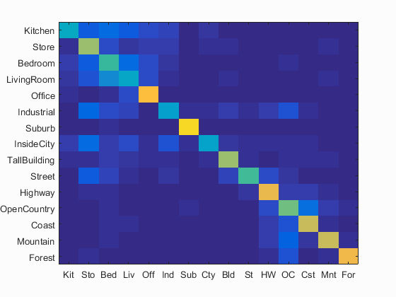
Scene classification results visualization
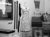
Accuracy (mean of diagonal of confusion matrix) is 0.614
| Category name | Accuracy | Sample training images | Sample true positives | False positives with true label | False negatives with wrong predicted label | ||||
|---|---|---|---|---|---|---|---|---|---|
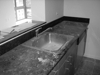
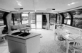
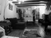
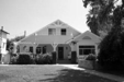
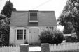
| Kitchen | 0.400 |  |
 |
 |
 |
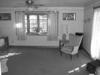 LivingRoom |
 Office |
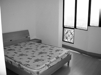
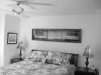
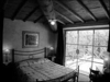
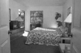
 Bedroom |
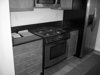 Bedroom |
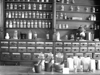
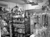
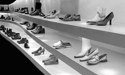
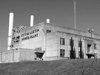
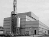
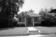
| Store | 0.650 |  |
 |
 |
 |
 Kitchen |
 InsideCity |
 Mountain |
 InsideCity |
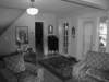
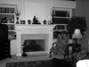
| Bedroom | 0.510 | 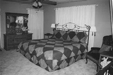 |
 |
 |
 |
 Mountain |
 Coast |
 LivingRoom |
 Store |
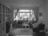
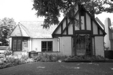
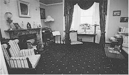
| LivingRoom | 0.390 | 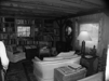 |
 |
 |
 |
 TallBuilding |
 Industrial |
 Bedroom |
 Bedroom |
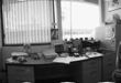
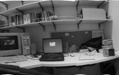
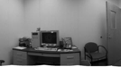
| Office | 0.840 | 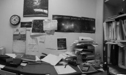 |
 |
 |
 |
 Store |
 LivingRoom |
 LivingRoom |
 Kitchen |
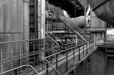
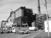
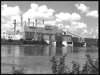
| Industrial | 0.350 | 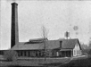 |
 |
 |
 |
 InsideCity |
 Store |
 Store |
 Store |
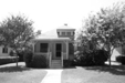
| Suburb | 0.910 | 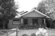 |
 |
 |
 |
 Street |
 LivingRoom |
 Bedroom |
 TallBuilding |
| InsideCity | 0.370 |  |
 |
 |
 |
 TallBuilding |
Store |
 TallBuilding |
 Suburb |
| TallBuilding | 0.650 |  |
 |
 |
 |
 InsideCity |
 Industrial |
 Store |
 Mountain |
| Street | 0.530 |  |
 |
 |
 |
 LivingRoom |
 Highway |
 Store |
 Highway |
| Highway | 0.790 |  |
 |
 |
 |
 Industrial |
 Coast |
 Street |
 Coast |
| OpenCountry | 0.580 |  |
 |
 |
 |
 Industrial |
 Highway |
 Highway |
 Forest |
| Coast | 0.720 |  |
 |
 |
 |
 OpenCountry |
 OpenCountry |
 Bedroom |
 Mountain |
| Mountain | 0.720 |  |
 |
 |
 |
 OpenCountry |
 OpenCountry |
 Highway |
 OpenCountry |
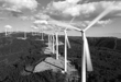
| Forest | 0.800 |  |
 |
 |
 |
OpenCountry |
 TallBuilding |
 Bedroom |
 OpenCountry |
| Category name | Accuracy | Sample training images | Sample true positives | False positives with true label | False negatives with wrong predicted label | ||||
Building a Vocabulary
I chose to attempt the extra credit where I experimented with different vocabulary sizes. For this, I chose to consider different vocabulary sizes ranging from 200-1000 with increments of 50. I also decided to consider a vocabulary size of just 10. The table below gives the results. I also chose to try with a vocab_size of 10 and for that I got 0.4373 accuracy. All the various vocabularies were tested with the bag of sifts features implementation with the nearest neighbor classifier detailed earlier.
| vocab_size = 200 | vocab_size = 250 | vocab_size = 300 | vocab_size = 350 | vocab_size = 400 | vocab_size = 450 | vocab_size = 500 | vocab_size = 550 | vocab_size = 600 | vocab_size = 650 | vocab_size = 700 | vocab_size = 750 | vocab_size = 800 | vocab_size = 850 | vocab_size = 900 | vocab_size = 950 | vocab_size = 1000 |
|---|---|---|---|---|---|---|---|---|---|---|---|---|---|---|---|---|
| 0.51930 | 0.51470 | 0.52870 | 0.53330 | 0.51530 | 0.51200 | 0.50200 | 0.51800 | 0.51200 | 0.50400 | 0.50600 | 0.50600 | 0.50130 | 0.51070 | 0.51070 | 0.51870 | 0.51870 |
I was a bit surprised because I was expecting a larger vocabulary size to lead to significantly higher accuracy, but I suspect a couple factors may have came into play with this. First, perhaps I was not going high enough. If I had more time, I would be interested in going up to 10000, for example. Second, perhaps I was skipping too much information with the Step values I was using. I maintained the same Step values of 8 and 4 that I mentioned previously when calculating these values, so perhaps with different Step values I would see a difference. The one thing that did fall under relatie expectations though was the result with the vocab_size of 10: It was definitely well below the others. This makes sense because we are using significantly less information to determine the classification. The one thing that's for sure though was that with larger vocab sizes, the processing took significantly longer. What became around 10 minutes of work perhaps easily became 15 or even 20. Literally about half a day at least as spent calculating all the vocabularies and using them with the bag of SIFT features.
General observations
Clearly the bags of SIFT features combined with the svm classifier worked pretty well. Of course, with lots of extra credit implementations, this accuracy could be improved further, but that's okay. Surprisingly different vocabulary sizes did not yield significant improvement with higher sizes (if anything, they wasted more time). Given more time, I would definitely consider even larger sizes to see if this trend is actually more local rather than global, especially considering that the small vocabulary size of 10 had significant detriment to the accuracy.