Project 4 / Scene Recognition with Bag of Words
The pipeline for this project was very straightforward, largely involving only two steps.
- Identify features.
- Classify.
For each of these steps, multiple design decisions are apparent. I will go into some options for each step and reasoning behind the decision made.
Identify Features
For the first step of the pipeline, several options are available. One of the simplest ways to represent an image is by scaling it down to a fixed size. Another is to identify SIFT features for each image, cluster these into a vocabulary, and create histograms for each image of the distribution of features in the clusters.
Tiny Images
Results of tiny images and nearest neighbor with an accuracy of 22.5%.
This is possibly the simplest forms of image representation. By scaling the image down to a fixed size, the feature dimension becomes much smaller and easier to classify. There are downsides to this approach. Downsampling the image throws away high-frequency features. This has the same effect as blurring, and may lead to decreased classification performance. On the other hand, this approach is performant in speed and memory. It is a simple process to complete, and only takes additional memory in the size of the input (e.g. the input image). The obvious free parameter with this approach is the fixed size of the resulting tiny images. Increasing or decreasing the size does not have a noticeable impact on the time it takes to transform the images to their intermediate representations. Contrary to this, increasing the size also increases the size of the feature space, something which may have a large impact on classification speed. When combined with a nearest neighbor classifier, the size does not have any noticeable impact on accuracy while the image size is larger than 16x16, however increasing the size from 16x16 to 32x32 more than quadruples the running speed. For these reason, the fixed size for optimal performance in terms of speed and accuracy was foudn to be 16x16.
Bag of SIFT Features
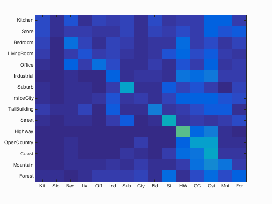
Results of bag of sift features and nearest neighbor with an accuracy of 52.1%.
Another option for representing images is by collecting SIFT features. This requires us to first form a vocabulary of clustered SIFT features from the test image space, then define a histogram of SIFT features for each image over these clusters. Anytime SIFT features are collected from an image, there are various free parameters that may be adjusted. One of these parameters, the step size, adjusts how often we find a feature in the current image. Because we find SIFT features twice for this representation, once for forming hte vocabulary and another time when forming the histograms, each of these step sizes may be different. For the first step, forming the vocabulary, we sample SIFT features from the images with a step size chosen to balance feature density and speed. After some experimentation, it was found that a step size ranging from 1 to 10 was most accurate. The larger the step size, the more SIFT features were collected, however the resulting vocabulary may suffer from insufficient examples. For this reason, a step size of 8 was chosen. Another parameter, the sampling rate, may also change the resulting clusters. A higher sampling rate means more features but longer times when clustering. Additionally, there is the risk of overtraining the clusters with a higher sampling rate. The time to cluster was not significantly changed with lower sampling rates until very few features per image remained. For this reason, all features were retained for clustering from each image. Lastly, the number of clusters may be adjusted for this step. Less clusters performed faster than more, however the time for the default number (200 clusters) was not significant when compared to other stages of the pipeline. For this reason, the number of clusters remained at the default, 200.
The next step in this representation includes forming a histogram of SIFT features using the newly formed vocabulary.
Again, the step size for this can be adjusted for alter performance.
In order to a representative sample of each image compared to the vocabulary, the step size was limited to a number less than the vocablary step size.
Starting at a step size of 8, it took nearly 11 minutes to get the feature histograms for just the training images.
Decreasing this to a step size of 4 reduced this to just under 9 minutes with only a minute drop in accuracy.
Another simple optimization was the use of parfor as opposed to the typical for loop in this function.
By parallelizing this function using MATLAB's Parallel Computing Toolbox, the execution time dropped from 9 minutes 5 minutes on my dual core machine.
Classify
For the final step of the pipeline, we have to classify using the representations we generated in the first step. The simplest way to do this is by assigning labels to the test images the label of their closest neighbor from the training images. Another form includes training a 1-vs-all support vector machine for each category in the set of unique labels.
k-Nearest Neighbors
The simplest form of classification in this project, k-nearest neighbors, or k-NN, measures the distance of a test feature to the space of training features and returns the mode label of the k neighbors with minimal distance. A simpler form of k-NN is 1-NN which simply returns the label of the closest label. The obvious free parameter in this case is k, the number of neighbors to look at. The number of distances measured remains fairly constant regardless of the specific value of k, therefore execution time didn't change significantly. When recording the accuracy of a tiny image representation being classified by k-NN, larger values of k were consistently associated with lower accuracies. The same trend was observed when classifying with the more complex bag of SIFT features. For these reasons, 1 was decided to be the best value of k.
Support Vector Machines
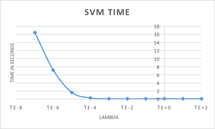
Effects of lambda on SVM classification speed.
The support vector machines, or SVMs, used in this project are specifically linear SVMs, and therefore are binary classifiers. When training, an SVM creates a hyperplane in the training instance space. A test instance is labeled based on which side of the hyperplane it rests on. Thus, by nature, a linear SVM may only classify between two distinct classes. In order to adapt them to a multi-class assignment, you can train a 1-vs-all SVM which will say if an instance is part of its category or not. After training a 1-vs-all SVM for each unique category, the most confident SVM is the classified label of the multi-class SVM.
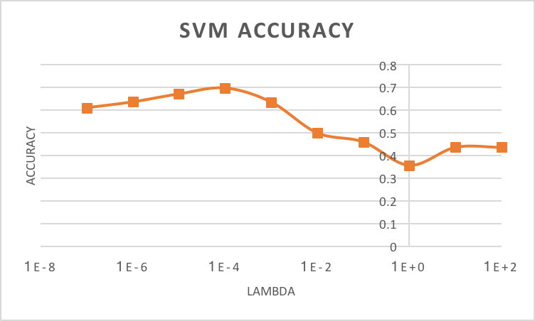
Effects of lambda on SVM classification accuracy.
When training, the most important free parameter to accuracy and runtime is lambda, which may range greatly. Typical values for this task lie between 1E-8 and 1E2. Through curiosity in the effects of various values of lambda, tests were performed with a wide range of lambdas on how they alter runtime and classification accuracy. These tests were performed with the same bag of SIFT features. As is evident by the SVM TIME graph on the right side, runtime is directly correlated with lambda. That is, as lambda decreases, so does runtime. Fortunately, runtime never exceeded 20 seconds with these tests. If you observe the SVM ACCURACY graph to the left, accuracy increased as did lambda, but only to a point. At values larger than 1E-4, accuracy began to drop significantly from 0.699 until settling at approximately 0.42. Fortunately, this value of 1E-4 also lines up with a very quick runtime, less than a second, and therefore was chosen as the optimal lambda value.
Results
In order to run in the allotted time of 10 minutes per configuration, some changes to the code had to be made. One such change was the vocabulary size and number of collected SIFT features per image. Reducing the size from 200 to 50 led to a speedup when building the bag of sift features. Additionally, only 220 SIFT features per image were retained, leading to a speedup when building the vocabulary itself. These changes reduced the runtime to within the acceptable range, however they hindered accuracy. With the current configuration and associated vocab.mat file, the slowest configuration is bag of features using a support vector machine at approximately 9 minutes. When using a tiny images representation and classifying with 1-nearest neighbor, an accuracy of 22.5% was achieved. By swapping the representation to a bag of SIFT features with 1-nearest neighbor, this accuracy increased to 52.1%. Only after classifying using the 15 1-vs-all support vector machines was the accuracy increased to 69.9%. At the end of this page you may find the fully generated webpage.
Conclusions
After analyzing the design decisions made throughout this project, several conclusions can be drawn. Most of the decisions were based on the accuracy-speed tradeoff. Nearest neighbor classifiers performed with a consistently lower accuracy when compared to support vector machines,however they often classified much quicker depending on certain free parameters. For the feature sets observed within this project, only the nearest neighbor was necessary to achieve an acceptable accuracy. Including more neighbors within classification increased execution time and was never found to be more accurate. Support vector machines consistently performed better to a nearest neighbor classifier, both in terms of accuracy across the board and often runtime too. Smaller lambda values consistently increased the runtime, but only increased accuracy up to a point. A happy medium was found where accuracy was high but runtime remained minimal. When deciding which feature set to use, a bag of SIFT features was consistently more accurate than tiny images, however the runtime became an issue. In order to meet the required time constraints, accuracy was conceded by reducing the size of the vocabulary. This smaller vocabulary allowed for the SIFT feature histograms to be formed faster than with its larger counterpart with only a 5% drop in accuracy.
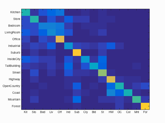
Bag of SIFTS with SVM results visualization
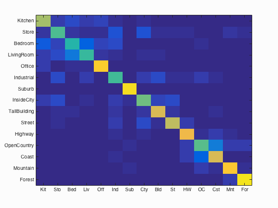
Accuracy (mean of diagonal of confusion matrix) is 0.699
| Category name | Accuracy | Sample training images | Sample true positives | False positives with true label | False negatives with wrong predicted label | ||||
|---|---|---|---|---|---|---|---|---|---|
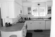
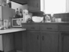
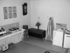
| Kitchen | 0.670 |  |
 |
 |
 |
 Office |
 InsideCity |
 Office |
 Bedroom |
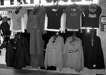
| Store | 0.540 | 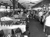 |
 |
 |
 |
 InsideCity |
 Industrial |
 Highway |
 Office |
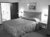
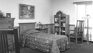
| Bedroom | 0.470 | 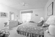 |
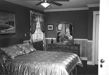 |
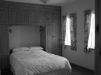 |
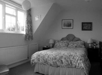 |
 LivingRoom |
 Store |
 LivingRoom |
 Office |
| LivingRoom | 0.500 |  |
 |
 |
 |
 Bedroom |
 Bedroom |
 Bedroom |
 Store |
| Office | 0.890 |  |
 |
 |
 |
 Kitchen |
 Bedroom |
 LivingRoom |
 Bedroom |
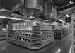
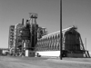
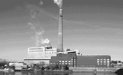
| Industrial | 0.530 |  |
 |
 |
 |
 Bedroom |
 Store |
 TallBuilding |
 Highway |
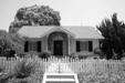
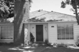
| Suburb | 0.930 |  |
 |
 |
 |
 Mountain |
 OpenCountry |
 OpenCountry |
 InsideCity |
| InsideCity | 0.590 |  |
 |
 |
 |
 Highway |
 Store |
 Street |
 LivingRoom |
| TallBuilding | 0.760 |  |
 |
 |
 |
 Industrial |
 InsideCity |
 Store |
 InsideCity |
| Street | 0.710 |  |
 |
 |
 |
 InsideCity |
 InsideCity |
 Highway |
 Store |
| Highway | 0.800 |  |
 |
 |
 |
 OpenCountry |
 Street |
 Mountain |
 InsideCity |
| OpenCountry | 0.550 |  |
 |
 |
 |
 Mountain |
 Industrial |
 Mountain |
Suburb |
| Coast | 0.750 |  |
 |
 |
 |
 OpenCountry |
 Highway |
 OpenCountry |
 Highway |
| Mountain | 0.860 |  |
 |
 |
 |
 Store |
 Forest |
OpenCountry |
 Highway |
| Forest | 0.940 |  |
 |
 |
 |
 Mountain |
 OpenCountry |
 Mountain |
 Mountain |
| Category name | Accuracy | Sample training images | Sample true positives | False positives with true label | False negatives with wrong predicted label | ||||