Methods

Tiny Images

Each image is taken and then downsized. This is used as the features with other classifiers, such as KNN once they become classified.

	image_feats = [];
	for i = 1:length(image_paths)
	    image = imread(image_paths{i});
	    image = imresize(image,[16 16]);
	    image = reshape(image,1,256);
	    image_feats(i,:) = image;
	end

Bag of Sifts

For this portion, a vocabulary is built to represent the training and testing image datasets, getting a bag of feature histogram. SIFT extracts features and clusters them. Vocabcular word size was 200.

In the code, an image is read in, and th VL dense sift featureing was used. Sift them randomly selects a set of features.

	imageLength = length(image_paths);
	SIFT = [];

	for i = 1:imageLength
	    image = imread(image_paths{i});
	    image = single(image);
	    [locations, SIFT_features] = vl_dsift(image,'fast','step',10);
	    randomPermutations = randperm(size(SIFT_features,2));
	    SIFT = [SIFT SIFT_features(:,randomPermutations(1:20))];
	end

	SIFT = single(SIFT);
	[vocab, assigned] = vl_kmeans(SIFT, vocab_size);

Here, in the bag of sift file, we read in an image, apply SIFT, and then get the distances and clustering to generate the model in order to try classifying test data.

	N = size(image_paths, 1);
	image_feats = zeros(N, vocab_size);

	for i = 1: N
	    image = imread(image_paths{i});
	    [location, sift_feats] = vl_dsift(single(image), 'fast', 'step', 5);

	    all_dist = vl_alldist2(single(sift_feats), vocab);
	    [sorted, index] = sort(all_dist, 2);

	    histogram = zeros(1, vocab_size);
	    for j = 1:size(index)
	        histogram(index(j, 1:5)) = histogram(index(j, 1:5))+[10 6 3 2 1];

	    end

	    histogram = histogram/norm(histogram,2);
	    image_feats(i,:) = histogram;

KNN

KNN deals in getting the nearest neighbors and then clustering them. Getting distances is quite straightforward through utilizing VLfeat.

	D = vl_alldist2(test_image_feats',train_image_feats');
	[B,I] = sort(D,2);
	permutations = I(:,1);
	predicted_categories = train_labels(permutations);

SVM

An SVM is a classifier than attempts to explode the data points to a higher dimension, and create a boundary line in this higher dimension (allowing for a more complex line), after which data/line is reduced to the normal dimension but keeping the complex linear seperator line. In this case, the line separates images within or ouside a category.

In this code, we get all the labels, and use VLfeat in order to do the SVM process. We choose the line of best confidence given the results.

	categories = unique(train_labels);
	num_categories = length(categories);

	lambda = 0.3;

	W = [];
	B = [];

	for i=1:num_categories
	    correctLabel = strcmp(categories(i),train_labels);
	    binaryLabel = ones(size(correctLabel)) .* -1;
	    binaryLabel(correctLabel) = 1;
	    [w,b] = vl_svmtrain(train_image_feats',binaryLabel',lambda);
	    W(i,:) = w;
	    B(i,:) = b;
	end


	for i=1:size(test_image_feats);
	    conf = [];
	    for j=1:num_categories
	        conf(j,:) = dot(W(j,:),test_image_feats(i,:)) + B(j,:);
	    end
	    [maxConf,index] = max(conf);
	    predicted_categories(i) = categories(index);
	end

	predicted_categories = predicted_categories';

Results

Base Case

Accuracy = .068

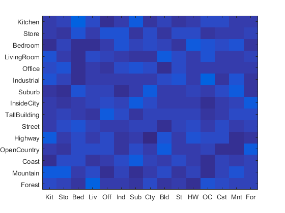
Tiny Images + KNN

Accuracy = .157

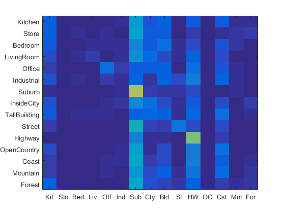
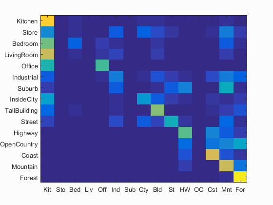
Bag of SIFT + KNN

Accuracy = .547

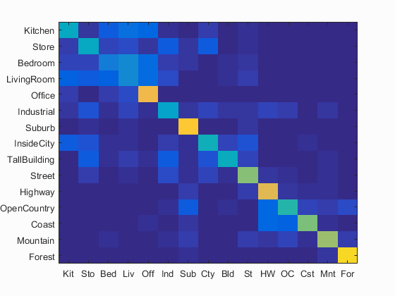
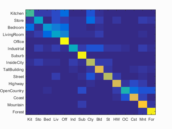
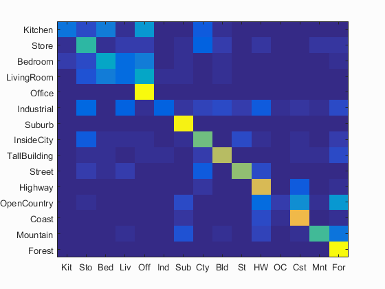
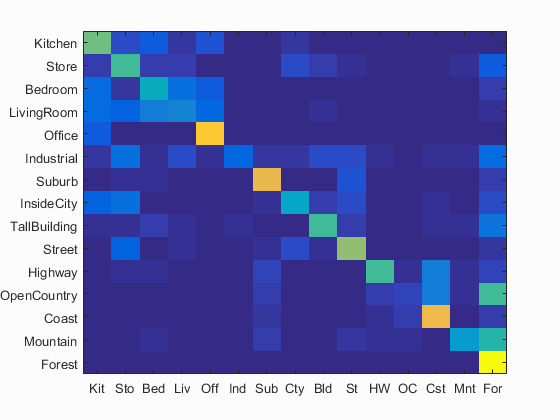
Bag of SIFT + SVM

Lambda = .0003	Lambda = .003	Lambda = .03	Lambda = .3
Accuracy = 0.661	Accuracy = 0.561	Accuracy = 0.525	Accuracy = 0.408

Scene classification best results visualization

Accuracy (mean of diagonal of confusion matrix) is 0.661

Category name	Accuracy	Sample training images		Sample true positives		False positives with true label		False negatives with wrong predicted label
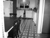
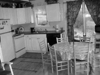
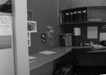
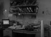
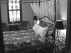
Kitchen	0.520					Bedroom	Store	Store	InsideCity
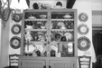
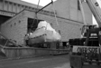
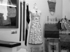
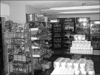
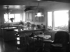
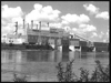
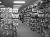
Store	0.390		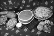			LivingRoom	Industrial	Industrial	LivingRoom
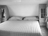
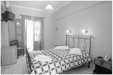
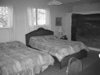
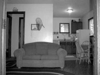
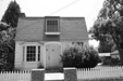
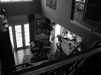
Bedroom	0.320					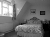LivingRoom	LivingRoom	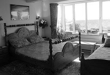LivingRoom	LivingRoom
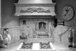
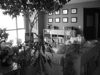
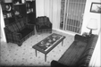
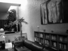
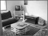
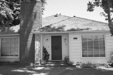
LivingRoom	0.360					Bedroom	Kitchen	Bedroom	Bedroom
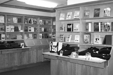
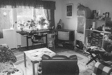
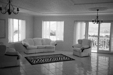
Office	0.990		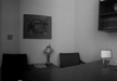			Kitchen	LivingRoom	Kitchen
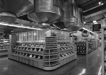
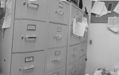
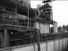
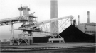
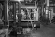
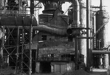
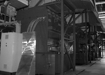
Industrial	0.410		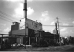			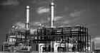Bedroom	LivingRoom	Store	InsideCity
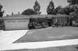
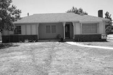
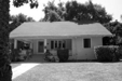
Suburb	0.970		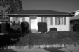			Industrial	OpenCountry	Street	InsideCity
InsideCity	0.690					Street	LivingRoom	Street	LivingRoom
TallBuilding	0.770					LivingRoom	Industrial	Kitchen	InsideCity
Street	0.690					InsideCity	Suburb	InsideCity	Mountain
Highway	0.750					Store	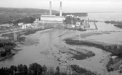Industrial	OpenCountry	Mountain
OpenCountry	0.460					Highway	Highway	Mountain	Coast
Coast	0.770					Highway	OpenCountry	Highway	Suburb
Mountain	0.870					OpenCountry	Highway	Store	Suburb
Forest	0.960					OpenCountry	Store	Mountain	Mountain
Category name	Accuracy	Sample training images		Sample true positives		False positives with true label		False negatives with wrong predicted label