Project 4 / Scene Recognition with Bag of Words
In this project we will examine some of the most simple methods to recognize scenes. Our specific task is to assign an accurate label to each scene: "forest", "bedroom", etc.
The project is comprised of 3 parts with each part demonstrating an approach slightly complicated than the previous ones. Throughout the 3 parts we will see that the accuracy of the algorithms improves from around 20% to 53% and ultimately to 68%.
There are two important things when it comes to image recognition: image representation and image classifications. For image representation in this project, we will use tiny images and bags of SIFT features, and for classification, we will use nearest neighbor and linear SVM. We will dive into more detail later on.
Part 1: Tiny images representation and nearest neighbor classifier
Accuracy achieved: 22.5%
The tiny images representation simply resizes the images to some small, fixed resolution, 16x16 pixels in this case. This will obviously lead to a loss of information, particularly the loss of the high frequencies in the images. However, it is very simple and the performance is not exactly bad. The code also makes the tiny images zero mean and unit length to improve the algorithm's weakness in dealing with intensity shifts. Doing this results in a roughly 2% improvement in accuracy.
For our nearest neighbor classifier, we simply find the nearest training example and take its label to assign to the test image. This method is fast to compute because it requires no preprocessing (no training). However, it is also susceptible to noise because if there's some noise in the training images, all of the nearest neighbors will also get classified to a wrong label.
Results
Accuracy (mean of diagonal of confusion matrix) is 0.225
Analysis: The algorithm runs very fast (it completes in less than 1 minute). The accuracy, although low, is surprisingly good for such a simple and seemingly bad method.
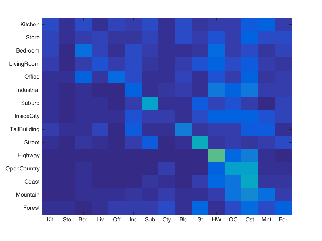
Part 2: Bag of SIFT representation and nearest neighbor classifier
Accuracy achieved: 53.1%
In this approach we reuse our nearest neighbor classifier, but instead of tiny images, we choose a better method: bag of SIFT features.
To do this, we first need to build a vocabulary. We get all the features from every training image and feed them into the function vl_kmeans(). This function will basically perform kmeans on our set of features and return the cluster centroids, which make up our vocab. The vocab size does make a big difference to the result accuracy. To see how this parameter affects the accuracy, check out the section Parameters Tuning.
After we've gotten the vocab, we can now represent images as histograms of visual words (or cluster centroids in our case). We again require the use of vl_dsift() to get sift features, then vl_alldist2() and min() to get the closest cluster centroids and increment their counts. At the end we normalize the histogram to ensure that an image doesn't have a different histogram just because it is larger with more SIFT features.
Results
Accuracy (mean of diagonal of confusion matrix) is 0.531
Analysis: The algorithm runs a lot slower due to training. However, the accuracy is much higher (about two times than the accuracy achieved by tiny images).
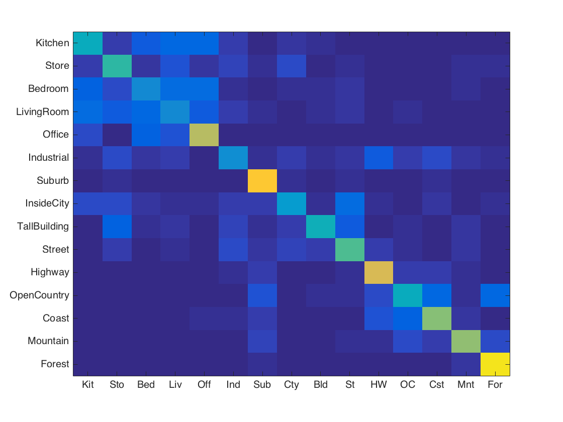
Part 3: Bag of SIFT representation and linear SVM classifier
Accuracy achieved: 68.0%
Finding nearest neighbor has high variance and low bias, the effect of which can be seen in its sensitivity to noise. A way to combat this is to use linear classifiers. Linear classifiers is on the opposite side of the spectrum with low variance and high bias. It also has weaknesses, however it fares much better in practice because it can deal with noise very efficiently.
In this particular project, we choose to implement 1-vs-all linear SVMS. We have 15 categories and we will train a linear SVM for each category. All 15 linear SVMs will be evaluated on each test image and the most confidently positive classifier wins. There's a free parameter lambda in this method, which can largely affect the results. The implementation is made relative simple with the use of vl_svmtrain(). We only need to compute a vector of 1 or -1 for each category, 1 means that the training image belongs to this category and -1 means it doesn't. After that, we simply use the weight vector W and the offset B returned by vl_svmtrain() to calculate the confidence scores. The max score indicates the category to which a test image belongs.
Results
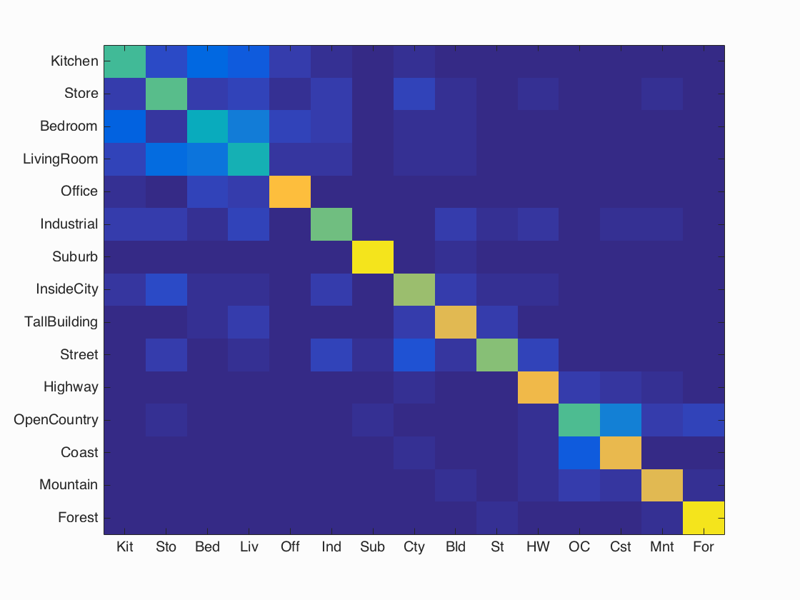
Accuracy (mean of diagonal of confusion matrix) is 0.680
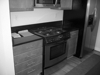
| Category name | Accuracy | Sample training images | Sample true positives | False positives with true label | False negatives with wrong predicted label | ||||
|---|---|---|---|---|---|---|---|---|---|
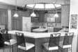
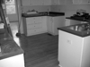
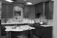
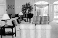
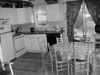
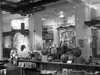
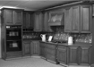
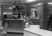
| Kitchen | 0.530 | 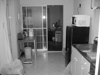 |
 |
 |
 |
 LivingRoom |
 Store |
 Store |
 Store |
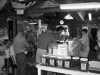
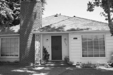
| Store | 0.560 |  |
 |
 |
 |
 LivingRoom |
Kitchen |
 LivingRoom |
 LivingRoom |
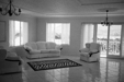
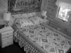
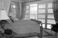
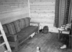
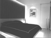
| Bedroom | 0.410 | 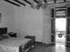 |
 |
 |
 |
 LivingRoom |
 InsideCity |
 LivingRoom |
 Store |
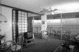
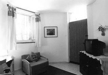
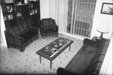
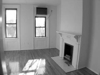
| LivingRoom | 0.440 | 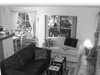 |
 |
 |
 |
 Bedroom |
 Kitchen |
 Store |
 Kitchen |
| Office | 0.830 |  |
 |
 |
 |
 Bedroom |
 Kitchen |
 Bedroom |
 LivingRoom |
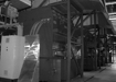
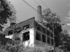
| Industrial | 0.580 | 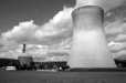 |
 |
 |
 |
 Kitchen |
 Coast |
 Coast |
 Forest |
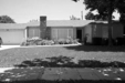
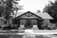
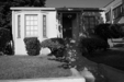
| Suburb | 0.950 | 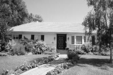 |
 |
 |
 |
 Street |
 Mountain |
 Store |
 InsideCity |
| InsideCity | 0.650 |  |
 |
 |
 |
 Kitchen |
 Kitchen |
 Kitchen |
 Store |
| TallBuilding | 0.780 |  |
 |
 |
 |
 Store |
 Bedroom |
 Street |
 InsideCity |
| Street | 0.610 |  |
 |
 |
 |
 TallBuilding |
 Forest |
 Industrial |
 Highway |
| Highway | 0.810 |  |
 |
 |
 |
 Store |
 Coast |
 OpenCountry |
 OpenCountry |
| OpenCountry | 0.540 |  |
 |
 |
 |
 Coast |
 Coast |
 Highway |
 Coast |
| Coast | 0.790 |  |
 |
 |
 |
 Office |
 OpenCountry |
 OpenCountry |
| Mountain | 0.780 |  |
 |
 |
 |
 OpenCountry |
 Street |
 Coast |
 OpenCountry |
| Forest | 0.940 |  |
 |
 |
 |
 OpenCountry |
Industrial |
Street |
 Mountain |
| Category name | Accuracy | Sample training images | Sample true positives | False positives with true label | False negatives with wrong predicted label | ||||
Parameters tuning
lambda: Approximately, the smaller the lambda, the higher the accuracy
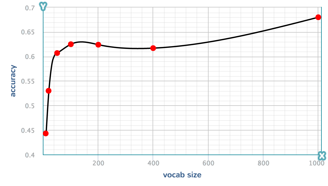
vocab size: If the vocab size is too small, we don't have enough "words" to describe an image. However, larger vocab sizes do not strictly mean higher accuracy. Higher vocab size will increase the variance but it also decreases the bias. In this case a vocab size of 1000 seems to work well but this may not be the case if we keep increasing the vocab size. I didn't test higher values because the 1000 vocab size already takes one hour to run.
| vocab | 10 | 20 | 50 | 100 | 200 | 400 | 1000 |
| accuracy | 0.443 | 0.530 | 0.607 | 0.625 | 0.624 | 0.617 | 0.680 |