Project 4 / Scene Recognition with Bag of Words
In Project 4, I had to implement Scene Recognition using a visual vocabulary, also known as a bag of words. The entire project entailed creating three different pipelines that utilized different methods of feature creation and classification. The following pipelines are listed below.
- Tiny Images and k-NN
- Bag of SIFT and k-NN
- Bag of SIFT and SVM
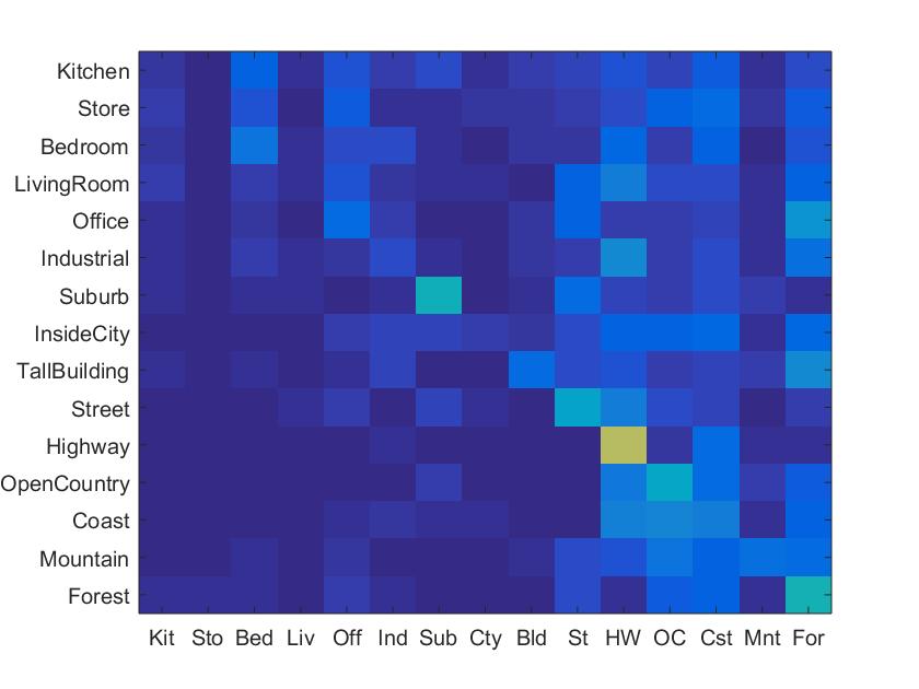
Part 1: Tiny Images and k-NN
The first pipeline utilized Tiny Image feature creation and k-NN classification. Tiny Image feature creation resizes and reshapes the original image into a [1 256] feature vector. Unlike SIFT feature creation, that makes features out of portions of an image, Tiny Image simply creates a feature from the entire image. This naturally loses alot of pertinent imformation, which explains the lower accuarcy. k-NN classifies images using Euclidean distances to find the nearest neighbors between the training and testing features passed into the function. k-NN trivially will take the minimum value from the acquired distances, and return that as the NN. However, increasing k allows for more distances to be considered. Each distance then votes, and the category with most votes is selected. In my code, I experimented with different k values, and found that after 15, the increase in accuracy slowly declined. Below is the code that I used to find the k minimum values.
k = 15;
...
for l = 1:k
        currentCat = train_labels(I(l), 1);
        for m = 1:num_categories
            vote = strcmp(currentCat, categories{m});
            if vote == 1
                voting_categories = [voting_categories, m];
            end
        end
end
The following is my best reported accuracy, with k = 15.

|
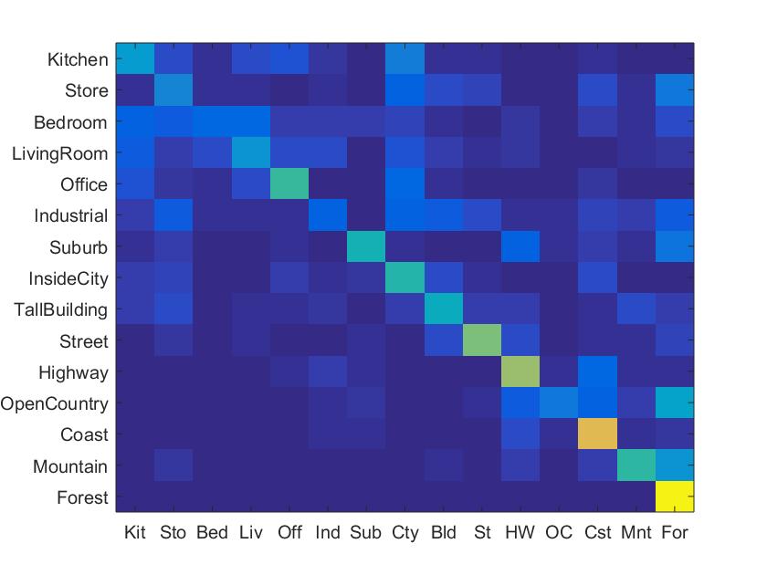
Part 2: Bag of SIFTs (Visual Vocabulary) and k-NN
The second pipeline changed the method to create features. Bag of SIFTs basically is implemented in two main steps. The first step is creating a visual vocabulary, where SIFT features are created from all the training images, then those features are clustered using the k-means algoritm. From this algoritm, we find a number of cluster centers, which are then saved as "visual words" in our vocabulary. The second step is then comparing the test image features against the vocabulary, and those closest are classified as the visual word. Those words are then compiled into a histogram and outputted to the k-NN classifiers. My SIFT step size for both build vocabulary and bag of sift sections was 16. While the TAs suggested a smaller step, I found that my accuarcy dropped substantially with a smaller step. This accuracy didn't waver with differnt k values for k-NN, so I kept it at 16. The following is a snippet from my build vocabulary showing how each word is created.
features = single(features);
[centers, assignments] = vl_kmeans(features, vocab_size);
vocab = centers';
The following is my reported accuracy, on the baseline of 45%. My best accuarcy with this pipeline increased when I increased the size of my vocabulary to 300, which was 46.2%. That pipeline ran over the 10 minute requirement.

|
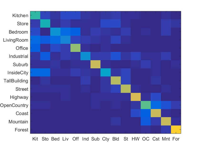
Part 3: Bag of SIFTs (Visual Vocabulary) and SVM
The third and final pipeline replaced the k-NN classification with SVM classification. SVM, short for support vector machine, are created for a specific category, like kitchen, so to recognize all features that are kitchen and not kitchen. In this sense, our SVMs are binary, returning either a 1 or 0 for the current feature being tested. I had to create 15 different SVMs for the 15 different categories. The SVMs were trained on a base set, creating W and B matrices (learned hyperplane parameters). These matrices could then be applied to the test features to recieve a confidence value, where the max confidence value would dictate how the image was classified. The lambda value causes the magnitude of the W output to remain small. The lambda value has a strong input on the accuarcy of the SVM classifier, and I found the greatest accuracy at lambda = 0.0001. The following is a snippet of how I trained my SVMs.
for i = 1:num_categories
    labels(1:num_features, 1) = -1;
    currentCategory = categories{i, 1};
    binaryLabels = strcmp(currentCategory, train_labels);
    indices = find(binaryLabels);
    for j = 1:size(indices, 1)
       currentIndex = indices(j, 1);
       labels(currentIndex, 1) = 1;
    end

    [W, B] = vl_svmtrain(single(train_image_feats'), labels', lambda);
    totalW = [totalW, W];
    totalB = [totalB, B];
end
The following is my reported accuracy, 56.9%. I found that like in the former pipeline, increasing my vocabulary size increased the accuarcy, where at a vocab_size = 300 and accuracy was 57.3%.

|