Project 4 / Scene Recognition with Bag of Words
Algorithm Description
Tiny Images Features
The Tiny Images classifier is quite simple, in that each image is just shrunk to a 16x16 image (without accounting for aspect ratio), and the pixel values of that 16x16 image are flattened into a 256 entry vector. This vector is then normalized to unit length and also made to have a zero mean.
Building the Vocabulary for Bag of Sifts
While buiding the vocabulary, to prevent overfitting as well as to decrease the runtime, half of the images are chosen at random to be sampled. From there, the SIFT features for each image are calculated, and 20 of those features are chosen to be added to the SIFT features pool. 20 was chosen as it provided the best accuracy for the memory usage. From there, the K-means clustering algorithm is performed, clustering the pool of SIFT features into "vocabulary size" clusters. The centers of these clusters are then returned as the dictionary. After testing, it became apparent that the performance increase due to a window size of 10 and the "fast" parameter being set for the SIFT algorithm outweighed the slight decrease in accuracy. Because of the randomness in the vocabulary building function, it is virtually impossible to recreate the exact same vocabulary. However, the difference in accuracy between different vocabularies should be 1 to 2% at a maximum.
Bag of SIFTs Feature
After the vocabulary is loaded into the script, the SIFT features for each image is calculated. After testing, it appeared that having a step size of 8 as well as the fast flag provided the best tradeoff in performance and accuracy. Then the Euclidean distance between each SIFT feature in each image and each visual word in the vocabulary is calculated. After this, the nearest words for each SIFT feature in each image are clustered into a histogram for each image. This histogram (with vocabulary size buckets) is then normalized (to add a level of size invariance) and used as the feature for its respective image.
Nearest Neighbor Classifier
This simple classifier calculates the Euclidean distance between the respective image's features and the training image's features. The predicted categories for each image feature are simply the categories that the repsective image's features are closest to in Euclidean distance.
SVM Classifier
After the categories are determined, for each category, the training features' labels are first checked to see if they are part of the specified category. Then, a matrix is created linking each training feature to a 1 if the feature is in the specified category and -1 otherwise. This is then passed into the SVM training function to create the W vector and the B value for the specific category.
Then, for each test image feature passed into the function, the feature is checked using the W and B values for each category. The category that yields the highest value in the function W*Feat + B is then the predicted category.
Results
Results for Tiny Images Features with Nearest Neighbor: Accuracy (mean of diagonal of confusion matrix) is 0.198
Bag of SIFT Features with Nearest Neighbor: Accuracy (mean of diagonal of confusion matrix) is 0.526
Best Results: Bag of SIFT Features with SVM
Accuracy (mean of diagonal of confusion matrix) is 0.639
Scene classification results visualization
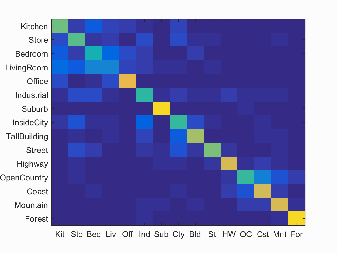
Accuracy (mean of diagonal of confusion matrix) is 0.639
| Category name | Accuracy | Sample training images | Sample true positives | False positives with true label | False negatives with wrong predicted label | ||||
|---|---|---|---|---|---|---|---|---|---|
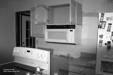
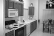
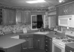
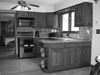
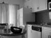
| Kitchen | 0.580 |  |
 |
 |
 |
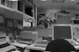
 Store |
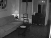
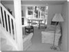
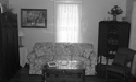 LivingRoom |
 Street |
 InsideCity |
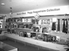
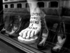
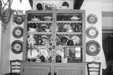
| Store | 0.560 |  |
 |
 |
 |
 LivingRoom |
 Kitchen |
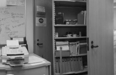
 Industrial |
 Highway |
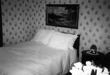
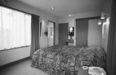
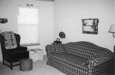
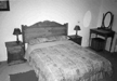
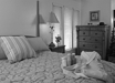
| Bedroom | 0.440 | 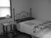 |
 |
 |
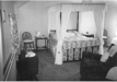 |
 Street |
 LivingRoom |
 Office |
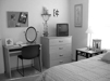 Kitchen |
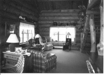
| LivingRoom | 0.260 | 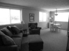 |
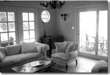 |
 |
 |
 Office |
 Bedroom |
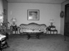 Bedroom |
 Bedroom |
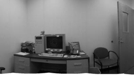
| Office | 0.790 | 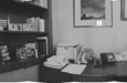 |
 |
 |
 |
 Bedroom |
 Kitchen |
 LivingRoom |
 Kitchen |
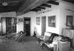
| Industrial | 0.490 | 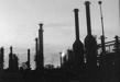 |
 |
 |
 |
 Bedroom |
 Kitchen |
 Store |
 Store |
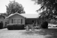
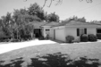
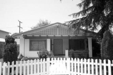
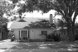
| Suburb | 0.920 | 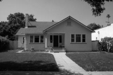 |
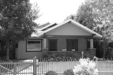 |
 |
 |
 TallBuilding |
 Highway |
 Store |
 LivingRoom |
| InsideCity | 0.510 |  |
 |
 |
 |
 Highway |
 TallBuilding |
 Suburb |
 Store |
| TallBuilding | 0.660 |  |
 |
 |
 |
 InsideCity |
 Street |
 InsideCity |
 Industrial |
| Street | 0.600 |  |
 |
 |
 |
 Industrial |
 InsideCity |
 Suburb |
 InsideCity |
| Highway | 0.760 |  |
 |
 |
 |
 Industrial |
 Street |
 Suburb |
 Store |
| OpenCountry | 0.510 |  |
 |
 |
 |
 Mountain |
 Coast |
 Coast |
 Highway |
| Coast | 0.740 |  |
 |
 |
 |
 OpenCountry |
 OpenCountry |
 Bedroom |
 Mountain |
| Mountain | 0.750 |  |
 |
 |
 |
 InsideCity |
 TallBuilding |
 Coast |
 Coast |
| Forest | 0.920 |  |
 |
 |
 |
 OpenCountry |
 OpenCountry |
 Store |
 Street |
| Category name | Accuracy | Sample training images | Sample true positives | False positives with true label | False negatives with wrong predicted label | ||||
In the end, the best-functioning pipeline was the linear SVM coupled with the Bag of SIFTs features. After testing, the classification of the linear SVM yielded the highest accuracy in comparison to the Nearest Neighbor classifier.