Caroline Paulus

Project 4 / Scene Recognition with Bag of Words

This project covers scene recognition using two different image representation types and two different classifiers. The scenes identified include nature examples such as mountain, forest, and coast, urban examples such as highway and tall building, and indoor examples such as kitchen and office. The accuracy of these recognition techniques ranges from approximately 20% using the less sophisticated representation type and classifier, to almost 70% using more advanced techniques.

I. Tiny Image Representation and Nearest Neighbor Classifier

The tiny image representation works by resizing each image to a very small (16 x 16) resolution. These resized images are used as training and test data. A collection of tiny training images, training labels, and tiny test images are passed to the nearest neighbor classifier. This classifier uses a pairwise distance calculator to find the training image with the most similar features to each test image, and labels the test image the same as the training image. My implementation actually returned more accurate results with 1 nearest neighbor, but the code is written in a way that would allow K to be a different value.

Results Visualization for Tiny Image/Nearest Neighbor Classifier

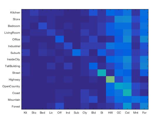
Accuracy (mean of diagonal of confusion matrix) is 0.201

Category name	Accuracy	Sample training images		Sample true positives		False positives with true label		False negatives with wrong predicted label
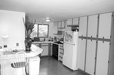
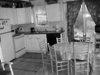
Kitchen	0.030					Suburb	Suburb	OpenCountry	Coast
Store	0.020					Kitchen	Forest	OpenCountry	Coast
Bedroom	0.090					LivingRoom	Kitchen	Coast	Coast
LivingRoom	0.070					Store	Highway	Coast	Street
Office	0.110					Mountain	Forest	Forest	TallBuilding
Industrial	0.090					Coast	TallBuilding	OpenCountry	Highway
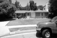
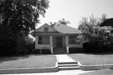
Suburb	0.170					OpenCountry	InsideCity	Bedroom	Kitchen
InsideCity	0.030					LivingRoom	Bedroom	Forest	Forest
TallBuilding	0.130					Kitchen	Office	Industrial	Highway
Street	0.430					LivingRoom	Suburb	Forest	Forest
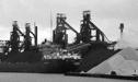
Highway	0.600					Coast	Industrial	OpenCountry	OpenCountry
OpenCountry	0.360					Kitchen	Street	Highway	Forest
Coast	0.440					Kitchen	Mountain	Mountain	Forest
Mountain	0.190					LivingRoom	OpenCountry	Forest	Office
Forest	0.260					LivingRoom	Street	OpenCountry	OpenCountry
Category name	Accuracy	Sample training images		Sample true positives		False positives with true label		False negatives with wrong predicted label

II. Bag of SIFT Representation and Nearest Neighbor Classifier

Since tiny images are a poor means of scene representation, the next step is to implement a more sophisticated technique called a bag of SIFT representation. SIFT stands for Scale-Invariant Feature Transform, and is an algorithm for detecting and identifying local features in images. This required first creating a vocabulary of visual words that features of images can be compared against. To achieve this, each image was sampled a number of times (I chose 100) to find SIFT features for that image, using a step size greater than 1 to avoid huge computation time (I chose 10). Once features were sampled from all the images, the cluster centroids were found using k-means clustering. These centroids are the visual word vocabulary.

My choice of 100 as a number of SIFT features to detect when building the vocabulary was somewhat arbitrary, but I also tested 220 (as suggested in the homework assignment) as a parameter. I found that 220 performed very slightly better using the nearest neighbor classifier (0.532 vs. 0.531) and slightly worse using the SVM classifier (0.687 vs. 0.693). This increase or decrease in performance was overall negligible and I chose to keep this parameter as 100.

The bag of SIFT representation algorithm goes through a set of images and generates a matrix of SIFT features for each. In this case, the step size is smaller (I chose five) to get a more fine-tuned result. I built a histogram with each location corresponding to to the visual words from the pre-determined vocabulary. For each SIFT feature in the image, I found the corresponding visual word closest to it and incremented that index in my histogram. The image features returned are a normalized histogram of visual words found in each image. (Note: the bag of SIFT representation takes several minutes to run.)

Results Visualization for Bag of SIFT/Nearest Neighbor Classifier

Accuracy (mean of diagonal of confusion matrix) is 0.531

Category name	Accuracy	Sample training images		Sample true positives		False positives with true label		False negatives with wrong predicted label
Kitchen	0.470		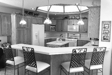			Bedroom	Industrial	LivingRoom	LivingRoom
Store	0.460					TallBuilding	InsideCity	Kitchen	Street
Bedroom	0.200					LivingRoom	Store	Office	LivingRoom
LivingRoom	0.400					Bedroom	Industrial	Industrial	Store
Office	0.850					LivingRoom	Bedroom	LivingRoom	LivingRoom
Industrial	0.330					Store	Highway	Store	Store
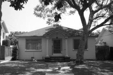
Suburb	0.870					Highway	TallBuilding	Coast	OpenCountry
InsideCity	0.400					Kitchen	Store	Street	Street
TallBuilding	0.400					Street	Industrial	Store	Forest
Street	0.560					InsideCity	InsideCity	Kitchen	Forest
Highway	0.650					Suburb	InsideCity	Industrial	Mountain
OpenCountry	0.400					Highway	Coast	Coast	Industrial
Coast	0.520					OpenCountry	Highway	Mountain	OpenCountry
Mountain	0.510					Street	Suburb	Forest	Highway
Forest	0.950					Mountain	Mountain	OpenCountry	Mountain
Category name	Accuracy	Sample training images		Sample true positives		False positives with true label		False negatives with wrong predicted label

III. Bag of SIFT Representation and 1-vs-all Linear SVM

To achieve an even better accuracy, a 1-vs-all Linear SVM can be used as a classifier. For each unique category (corresponding to the scene labels), a set of binary training labels is found by making the labels matching the current category +1 and every other value -1. A SVM is trained using the training data and modified labels (as well as a parameter lambda, to be discussed in more detail below), and returns a set of weights and biases such that the score W' * X(:, i) + B has the sign of labels(i) for all i (from MATLAB vl_svmtrain documentation). After performing this for each category and storing the weights and biases, the best category for each test image can be found by finding the confidence score using W*X + B, and returning the categories associated with the most confident scorings.

The parameter lambda made a huge difference in the accuracy of the SVM classifier. I found that a very small value for lambda, 0.0001, performed the best, with an accuracy of 0.693. Making lambda smaller (0.00001) resulted in an accuracy of 0.657, and as lambda got larger, the accuracy quickly decreased. The following are different values of lambda and their corresponding accuracies: 0.001 = 0.603, 0.01 = 0.469, 0.1 = 0.521, 1 = 0.315.

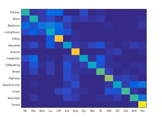
Results Visualization for Bag of SIFT/1-vs-all Linear SVM Classifier

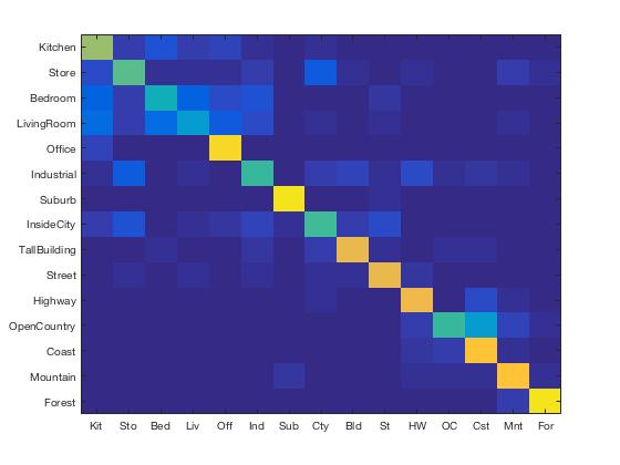
Accuracy (mean of diagonal of confusion matrix) is 0.693

Category name	Accuracy	Sample training images		Sample true positives		False positives with true label		False negatives with wrong predicted label
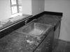
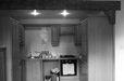
Kitchen	0.650					InsideCity	Office	Office	Bedroom
Store	0.560					LivingRoom	Bedroom	TallBuilding	Bedroom
Bedroom	0.430					Kitchen	LivingRoom	Industrial	Kitchen
LivingRoom	0.330					Bedroom	Street	Bedroom	Office
Office	0.920					LivingRoom	Kitchen	Kitchen	Kitchen
Industrial	0.510					Highway	Bedroom	OpenCountry	InsideCity
Suburb	0.950					Mountain	Mountain	OpenCountry	Street
InsideCity	0.520					Store	Industrial	Office	Industrial
TallBuilding	0.790					Industrial	Industrial	LivingRoom	Street
Street	0.790					Bedroom	LivingRoom	Highway	TallBuilding
Highway	0.800					OpenCountry	Industrial	Coast	Coast
OpenCountry	0.500					TallBuilding	Highway	Coast	Mountain
Coast	0.850					OpenCountry	Highway	Bedroom	OpenCountry
Mountain	0.850					Bedroom	OpenCountry	Suburb	LivingRoom
Forest	0.940					Mountain	TallBuilding	Mountain	Mountain
Category name	Accuracy	Sample training images		Sample true positives		False positives with true label		False negatives with wrong predicted label