Project 4 / Scene Recognition with Bag of Words
Introduction
The purpose of this project was to cover the topic of image recognition, a problem in computer vision that aims to distinguish classes of scenes. In the case of this project, the scene classes were as follows, ordered by similarity:
- Kitchen
- Store
- Bedroom
- LivingRoom
- Office
- Industrial
- Suburb
- InsideCity
- TallBuilding
- Street
- Highway
- OpenCountry
- Coast
- Mountain
The core approaches for image recognition in this project are based around the idea of extracting strong, distinguishing features from an image to describe image classes to machine learning algorithms. By training machine learning algorithms with the features labeled by these image classes, the algorithm is eventually able to classify a given set of features corresponding to an image without a label. Specifically for the project, the following approaches were used in the image recognition pipeline:
Feature Extraction
- Tiny Image: downsizing an image to a much smaller resolution, using pixel intensity values as features.
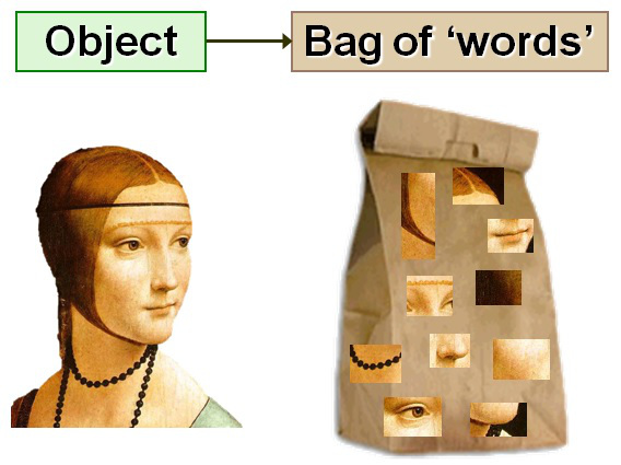
- Bag of SIFT Features: creating a set of SIFT features for a given image, using the SIFT descriptors as features.
Classifiers
- Nearest Neighbor: given some set of unknown features (an unlabeled datapoint), look at the most similar known datapoint to classify the unknown datapoint.
- 1 vs. All Support Vector Machines: for each class, train a binary support vector machine that separates positive datapoints (of a class) from negative datapoints (of a class). When presented with an unknown datapoint, find which class's support vector machine most strongly claims the datapoint as positive (belonging to that class).
Tiny Image Features + Nearest Neighbor
The simplest version of the pipeline resized the images to 16x16 and used the pixel intensity values from the resulting image to create a point for the nearest neighbor algorithm. The results were:
Accuracy (mean of diagonal of confusion matrix) is 0.191
The poor results were unsurprising, considering the nature of the tiny image approach to features. By resizing an image to a very small resolution, the algorithm still maintains the general idea of the image and preserves the low frequencies, but potentially important details at high frequencies are lost. With the loss of high frequencies, it becomes very difficult for the algorithm to distinguish between similar scenes when details are lost.
Bag of SIFT + Nearest Neighbor
To combat the poor image generalization and lossy nature of the tiny image's features, the bag of SIFT method was used instead. The accuracy was significantly improved:
Accuracy (mean of diagonal of confusion matrix) is 0.544
The improvement in the results were likely due to the vastly superior features that the bag of SIFT method provided. SIFT keypoints are much better at extracting unique and distinguishing points of interest of a scene and providing a robust descriptor that allows for that point to be matched across different scenes for similarity. With such a large improvement from the feature extraction, the focus shifted towards the learning algorithm, nearest neighbor. Nearest neighbor is a very intuitive learning algorithm when given the assumption that datapoints close together exhibit similar features and therefore belong to a similar class. However, by selecting just one neighbor, the algorithm is very susceptible to noise and can therefore overfit data aggressively.
Bag of SIFT + Support Vector Machine
Finally, the last major improvement of the standard scene recognition pipeline was to use support vector machines to learn and classify the features. The classification performance was once again improved:
Accuracy (mean of diagonal of confusion matrix) is 0.649
With an improved learning algorithm, the pipeline was able to identify scenes even more accurately, even with some noise. Even so, there were still difficulties distinguishing between the store, bedroom, and living room. This made logical sense, since those scenes exhibit very similar visual cues and objects that possess many similar points of interest.
Bonus: Tuning Parameters with a Validation Set
To tune the parameters for the bag of SIFT + SVM setup, a validation set was used. A Python script, pick_validation_set.py, was written to randomly sample from the test set to create the validation set. The following validation set was used for tuning:
../data/test/Bedroom/image_0158.jpg
../data/test/Bedroom/image_0176.jpg
../data/test/Bedroom/image_0037.jpg
../data/test/Bedroom/image_0196.jpg
../data/test/Coast/image_0177.jpg
../data/test/Coast/image_0124.jpg
../data/test/Coast/image_0349.jpg
../data/test/Coast/image_0331.jpg
../data/test/Forest/image_0198.jpg
../data/test/Forest/image_0101.jpg
../data/test/Forest/image_0196.jpg
../data/test/Forest/image_0319.jpg
../data/test/Highway/image_0184.jpg
../data/test/Highway/image_0220.jpg
../data/test/Highway/image_0232.jpg
../data/test/Highway/image_0211.jpg
../data/test/Industrial/image_0178.jpg
../data/test/Industrial/image_0045.jpg
../data/test/Industrial/image_0123.jpg
../data/test/Industrial/image_0245.jpg
../data/test/InsideCity/image_0002.jpg
../data/test/InsideCity/image_0251.jpg
../data/test/InsideCity/image_0297.jpg
../data/test/InsideCity/image_0048.jpg
../data/test/Kitchen/image_0071.jpg
../data/test/Kitchen/image_0057.jpg
../data/test/Kitchen/image_0097.jpg
../data/test/Kitchen/image_0147.jpg
../data/test/LivingRoom/image_0126.jpg
../data/test/LivingRoom/image_0114.jpg
../data/test/LivingRoom/image_0156.jpg
../data/test/LivingRoom/image_0160.jpg
../data/test/Mountain/image_0186.jpg
../data/test/Mountain/image_0254.jpg
../data/test/Mountain/image_0297.jpg
../data/test/Mountain/image_0146.jpg
../data/test/Office/image_0180.jpg
../data/test/Office/image_0089.jpg
../data/test/Office/image_0047.jpg
../data/test/Office/image_0121.jpg
../data/test/OpenCountry/image_0008.jpg
../data/test/OpenCountry/image_0109.jpg
../data/test/OpenCountry/image_0189.jpg
../data/test/OpenCountry/image_0164.jpg
../data/test/Store/image_0296.jpg
../data/test/Store/image_0259.jpg
../data/test/Store/image_0300.jpg
../data/test/Store/image_0166.jpg
../data/test/Street/image_0161.jpg
../data/test/Street/image_0232.jpg
../data/test/Street/image_0042.jpg
../data/test/Street/image_0106.jpg
../data/test/Suburb/image_0061.jpg
../data/test/Suburb/image_0213.jpg
../data/test/Suburb/image_0182.jpg
../data/test/Suburb/image_0138.jpg
../data/test/TallBuilding/image_0138.jpg
../data/test/TallBuilding/image_0136.jpg
../data/test/TallBuilding/image_0088.jpg
../data/test/TallBuilding/image_0221.jpg
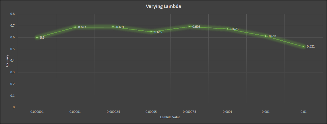
The main parameter adjusted was lambda for the SVM, and the following are visualisations of how the experiments performed.
0.000001
Getting paths and labels for all train and test data
Using bag of sift representation for images
No existing visual word vocabulary found. Computing one from training images
Using support vector machine classifier to predict test set categories
Creating results_webpage/index.html, thumbnails, and confusion matrix
Accuracy (mean of diagonal of confusion matrix) is 0.600

0.00001
Getting paths and labels for all train and test data
Using bag of sift representation for images
Using support vector machine classifier to predict test set categories
Creating results_webpage/index.html, thumbnails, and confusion matrix
Accuracy (mean of diagonal of confusion matrix) is 0.687

0.000025
Getting paths and labels for all train and test data
Using bag of sift representation for images
No existing visual word vocabulary found. Computing one from training images
Using support vector machine classifier to predict test set categories
Creating results_webpage/index.html, thumbnails, and confusion matrix
Accuracy (mean of diagonal of confusion matrix) is 0.691

0.00005
Getting paths and labels for all train and test data
Using bag of sift representation for images
Using support vector machine classifier to predict test set categories
Creating results_webpage/index.html, thumbnails, and confusion matrix
Accuracy (mean of diagonal of confusion matrix) is 0.649

0.000075
Getting paths and labels for all train and test data
Using bag of sift representation for images
Using support vector machine classifier to predict test set categories
Creating results_webpage/index.html, thumbnails, and confusion matrix
Accuracy (mean of diagonal of confusion matrix) is 0.693

0.0001
Getting paths and labels for all train and test data
Using bag of sift representation for images
Using support vector machine classifier to predict test set categories
Creating results_webpage/index.html, thumbnails, and confusion matrix
Accuracy (mean of diagonal of confusion matrix) is 0.673

0.001
Getting paths and labels for all train and test data
Using bag of sift representation for images
Using support vector machine classifier to predict test set categories
Creating results_webpage/index.html, thumbnails, and confusion matrix
Accuracy (mean of diagonal of confusion matrix) is 0.611

0.01
Getting paths and labels for all train and test data
Using bag of sift representation for images
Using support vector machine classifier to predict test set categories
Creating results_webpage/index.html, thumbnails, and confusion matrix
Accuracy (mean of diagonal of confusion matrix) is 0.522
From the data above, it is clear that there exists a sweet spot between 0.00001 and 0.0001 lambda values, and from the experiments, the best value was 0.00075, providing an accuracy value of 0.693.
Bonus: Varying Vocabulary Size
All of the previous results used only 200 vocabulary words. This part of the project aimed to experiment with the effect of the vocabulary size on classification and recognition performance.
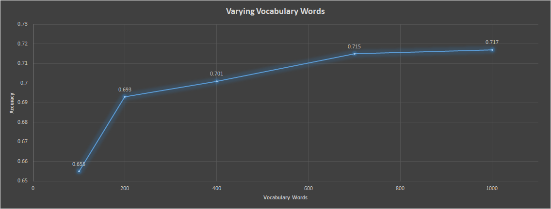
From the data above, the vocabulary size clearly affects accuracy in a positive way as the vocabulary size gets larger. However, the time it takes to complete the pipeline grows much faster than a linear relationship, so there comes a point above 700 words or so that the accuracy for time tradeoff is not worth it. In fact, the experiment was run on 5000 words, and after 4 hours, the code was still running. In conclusion, there is a optimal spot that trades off well between accuracy and time around 700 words.
Best Results
After all the experimentation, here are the best results, with an accuracy of 0.717.
Scene classification results visualization
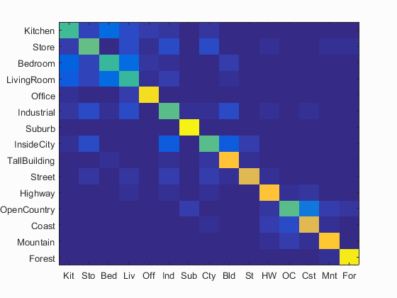
Accuracy (mean of diagonal of confusion matrix) is 0.717
| Category name | Accuracy | Sample training images | Sample true positives | False positives with true label | False negatives with wrong predicted label | ||||
|---|---|---|---|---|---|---|---|---|---|
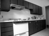
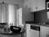
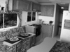
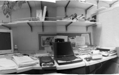
| Kitchen | 0.520 | 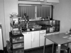 |
 |
 |
 |
 Bedroom |
 Bedroom |
 Bedroom |
 LivingRoom |
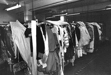
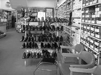
| Store | 0.570 |  |
 |
 |
 |
 InsideCity |
 Street |
 LivingRoom |
 LivingRoom |
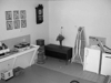
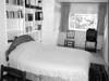
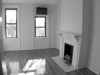
| Bedroom | 0.500 |  |
 |
 |
 |
 LivingRoom |
 Kitchen |
 Kitchen |
 LivingRoom |
| LivingRoom | 0.510 |  |
 |
 |
 |
 Street |
 Store |
 Bedroom |
 Store |
| Office | 0.930 |  |
 |
 |
 |
 LivingRoom |
Industrial |
 Kitchen |
 LivingRoom |
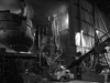
| Industrial | 0.560 | 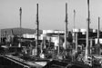 |
 |
 |
 |
 Highway |
 InsideCity |
 TallBuilding |
 TallBuilding |
| Suburb | 0.980 |  |
 |
 |
 |
 LivingRoom |
 Coast |
 OpenCountry |
 InsideCity |
| InsideCity | 0.560 |  |
 |
 |
 |
 Street |
 TallBuilding |
 Industrial |
 Industrial |
| TallBuilding | 0.850 |  |
 |
 |
 |
 InsideCity |
 Bedroom |
 Industrial |
 LivingRoom |
| Street | 0.770 |  |
 |
 |
 |
 Highway |
 InsideCity |
 InsideCity |
Store |
| Highway | 0.850 |  |
 |
 |
 |
 Coast |
 OpenCountry |
 Coast |
 Industrial |
| OpenCountry | 0.550 |  |
 |
 |
 |
 Mountain |
 Industrial |
 Coast |
 Highway |
| Coast | 0.780 |  |
 |
 |
 |
 OpenCountry |
 TallBuilding |
 OpenCountry |
 OpenCountry |
| Mountain | 0.860 |  |
 |
 |
 |
 Coast |
 Forest |
 LivingRoom |
 TallBuilding |
| Forest | 0.960 |  |
 |
 |
 |
 Store |
 Mountain |
 Store |
 Mountain |
| Category name | Accuracy | Sample training images | Sample true positives | False positives with true label | False negatives with wrong predicted label | ||||