Project 4 / Scene Recognition with Bag of Words
This project consisted of writing 2 feature detectors and 2 classifiers. I then used different combinations of these feature detectors and classifiers to recognize scenes.
Feature Detectors
The first feature detector I wrote was get_tiny_images. In get tiny images I iterated over the images and resized them to be 16x16 images. I then reshaped and normalized them so retain comparability.
The second feature detector I wrote was get_bags_of_sifts. For bags of sifts I had to first construct a vocabulary. I created a vocabulary by iterating over the images and finding the sift features of the image with vlfeat’s vl_dsift. I used a step of 8 and size of 4 as these numbers provided the best initial results. I performed vlfeat’s kmean on all of the features obtained from all of the images. Kmeans clustered the feature and returned a centroid feature for each cluster. I then used this centroid feature as my vocabulary words to compare test features to. I then was able to continue with get_bags_of_sifts. I used vlfeat’s vl_kdtreebuild to build a KD-tree from the vocab. I then iterated over the images and found the sift features for each image using the vl_dsift again. I used the same parameters here as in build vocabulary. I used these features to do a query of the kdtree and create a histogram to show how often a cluster was used for each image. I then normalized the histogram so that image size did not affect the categorization.
Classifiers
The first classifier I wrote was nearest_neighbors_classify. For nearest neighbors I calculated the distance between the test image features and the train image features and found the minimum distance to a train feature from a test feature. I used that train feature to then derive the label of the test feature from the train labels.
The second classifier I wrote was svm_classify, a support vector machine. Here I iterated over the categories and for each category I created a 1 vs. all labeling system where the images in the focused category were denoted by 1 and the images not in the focused category were denoted by -1. I then used this labeling system to create a svm using vlfeat’s vl_svm from the train image features. This svm allowed for a varying value of lambda. I chose a lambda value of 0.0001 because values 0.001 and 0.00001 both resulted in lower accuracies. I then iterated over the test image features and derived a confidence for each category and image. I created this confidence from the w and b values obtained from the svm (W*X + B). I then found the max category confidence for each feature and returned the predicted categories.
Accuracies
|
Tiny Images and Nearest Neighbor |
20.1% |
|
Bag of SIFT and Nearest Neighbor |
45.3% |
|
Bag of SIFT and 1 vs. All Linear SVM |
59.6% |
Extra Credit- Experimenting with different vocabulary sizes
While doing the required parts of the assignment I became very interested in how much the accuracies could change with just a new vocabulary. For example, if I ran the bag of sifts and svm with one vocab I could get a +/-0.05% difference on the accuracy. I decided to learn more about the vocabulary impact by doing this extra credit. I have ran both the svm and the nearest neighbors algorithm with varying vocabulary sizes used in bag of sifts. Run time increased greatly when incrementing the vocabulary size. As expected, the Bag of Sifts and Nearest Neighbor accuracies are consistantly below the Bag of Sifts and SVM accuracies. However, it is interesting to note that they follow a very similar arch with steady increase between 10 and 100 and decrease after. This is most likely due to an increase in words that do not add in categorization. For example, features that are green and of a certain texture and features that are brown and of a certain texture might be both classified as "trees" whereas with more words they might be broken down into leaves and bark which are easier to hallucinate in images without trees.

Scene classification results visualization
(Based on highest non-extra credit run)
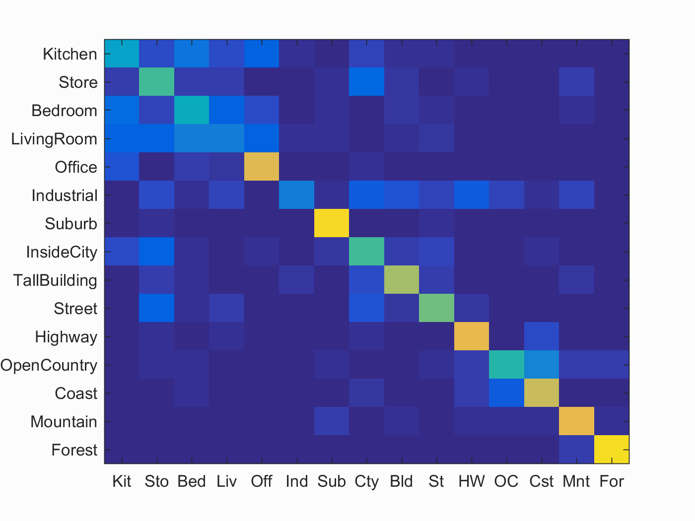
Accuracy (mean of diagonal of confusion matrix) is 0.596
| Category name | Accuracy | Sample training images | Sample true positives | False positives with true label | False negatives with wrong predicted label | ||||
|---|---|---|---|---|---|---|---|---|---|
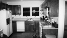
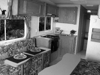
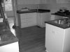
| Kitchen | 0.360 | 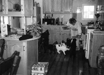 |
 |
 |
 |
 LivingRoom |
 Coast |
 Bedroom |
 Store |
| Store | 0.530 |  |
 |
 |
 |
 Street |
 Street |
 Forest |
 Bedroom |
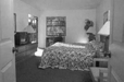
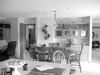
| Bedroom | 0.420 |  |
 |
 |
 |
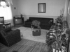
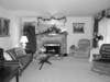 LivingRoom |
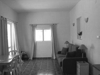 LivingRoom |
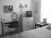 LivingRoom |
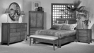 Street |
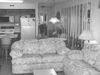
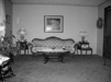
| LivingRoom | 0.230 |  |
 |
 |
 |
 Bedroom |
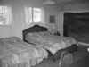 Bedroom |
 Industrial |
 Mountain |
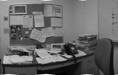
| Office | 0.770 |  |
 |
 |
 |
 InsideCity |
 Kitchen |
 LivingRoom |
 Kitchen |
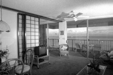
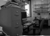
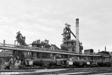
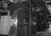
| Industrial | 0.220 |  |
 |
 |
 |
 LivingRoom |
 Kitchen |
 TallBuilding |
 LivingRoom |
| Suburb | 0.910 |  |
 |
 |
 |
 OpenCountry |
 Store |
 Street |
 Mountain |
| InsideCity | 0.520 |  |
 |
 |
 |
 TallBuilding |
 TallBuilding |
 Store |
 TallBuilding |
| TallBuilding | 0.670 |  |
 |
 |
 |
 Street |
 Mountain |
 Mountain |
 Industrial |
| Street | 0.590 |  |
 |
 |
 |
 Bedroom |
 Industrial |
 Suburb |
 InsideCity |
| Highway | 0.790 |  |
 |
 |
 |
 TallBuilding |
 OpenCountry |
 OpenCountry |
 LivingRoom |
| OpenCountry | 0.480 |  |
 |
 |
 |
 Coast |
 Mountain |
 TallBuilding |
 Coast |
| Coast | 0.730 |  |
 |
 |
 |
 OpenCountry |
 Highway |
 InsideCity |
 OpenCountry |
| Mountain | 0.790 |  |
 |
 |
 |
Suburb |
Industrial |
 Coast |
 TallBuilding |
| Forest | 0.930 |  |
 |
 |
 |
Store |
 OpenCountry |
 Mountain |
 Street |
| Category name | Accuracy | Sample training images | Sample true positives | False positives with true label | False negatives with wrong predicted label | ||||