Project 4 / Scene Recognition with Bag of Words
This project evaluates different methods and pipelines for doing scene recognition using a classic bag of words approach.Tiny Images and Nearest Neighbor
This is the simplest approach. The features are input images scaled down to 16x16 pixel and then zero meaned and normalized to a unit vector.
image = imresize(image, [image_size image_size]);
image = image(:);

% zero mean and unit length
image = double(image);
image = image / sum(image);
image = image - mean(image);

image_feats(i,:) = image;
By calculating the K-Nearest Neighbors for a test image to the training images and using the most common label of the neighbors we can predict the label of the test image. Using this approach with K=1 I got 0.199 accuracy.
K = 1;
[D, I] = pdist2(train_image_feats, test_image_feats, 'euclidean','Smallest',K);
if K > 3
    I = mode(I);
end
predicted_categories = train_labels(I);
Bag of SIFT and Nearest Neighbor
By extracting features using SIFT rather than just miniturizations the accuracy will improve further. This is done in two steps.
First we build a vocabulary of less dense SIFT features from all our training images. These are then clustered into K clusters.
FEATURE_STEP_SIZE=5;
FEATURE_SIZE=3;

all_features = [];
for i=1:size(image_paths)
    path = image_paths{i};
    image = single(imread(path));
    [positions, features] = vl_dsift(image, 'fast', 'Step', FEATURE_STEP_SIZE, 'Size', FEATURE_SIZE);
    % features is d x N
    all_features = [all_features, features];
end

[centers, assignments] = vl_kmeans(single(all_features), vocab_size);
vocab = centers';
K here is the given parameter vocab_size. I use a FEATURE_STEP_SIZE=5 and FEATURE_SIZE=3 this gives a balance between speed and accuracy.
The next step is to extract dense featurs from the test image and their nearest neighbors in amongst the training image vocabulary.
path = image_paths{i};
image = single(imread(path));
[positions, features] = vl_dsift(image, 'Fast', 'Step', FEATURE_STEP_SIZE, 'Size', FEATURE_SIZE);
features = double(features);

[D, I] = pdist2(vocab, features', 'euclidean','Smallest', 1);
% [I, D] = vl_kdtreequery(forest, vocab', features);

% create histogram
hist = zeros([vocab_size 1]);
for j=1:size(I, 2)
		cluster = I(j);
		hist(cluster) = hist(cluster) + 1;
end
hist = hist / sum(hist);
image_feats = [image_feats, hist];
Experimentally I found that FEATURE_STEP_SIZE=5 and FEATURE_SIZE=3 gave a good balance between speed and accuracy. This yields an accuracy of 0.509.
Bag of SIFT and Linear SVM
This is the final improvement using 1 vs all linear SVM classifiers. That is, for each of the 15 categories a SVM is trained to classify between "category X" and "not category X". Then for each test image all SVM give their prediction and the most certain result is used.
% build classifiers
W = [];
B = [];
for i=1:num_categories
    matching_indices = strcmp(categories(i), train_labels);
    labels = ones([N 1]) * -1;
    labels(matching_indices) = 1;
    labels = double(labels);
    [w b] = vl_svmtrain(train_image_feats', labels, LAMBDA);
    W = [W, w];
    B = [B, b];
end

% classify data
M = size(test_image_feats, 1);
predicted_categories = cell(M, 1);
for i=1:M
    Y = W' * test_image_feats(i,:)' + B';
    [M, label_id] = max(Y);
    predicted_categories{i} = categories{label_id};
end
predicted_categories
LAMBDA = 0.000001 was experimentally showing to give the best result together with FEATURE_STEP_SIZE=2 and FEATURE_SIZE=3 when extracting the dense SIFT features from the test images. The resulting accuracy was 0.709 and the result is vizualized below. This however is a bit slow, and by setting FEATURE_STEP_SIZE=5 we decrease the time drastically but still get an acceptable accuracy of 0.68.
Scene classification results visualization
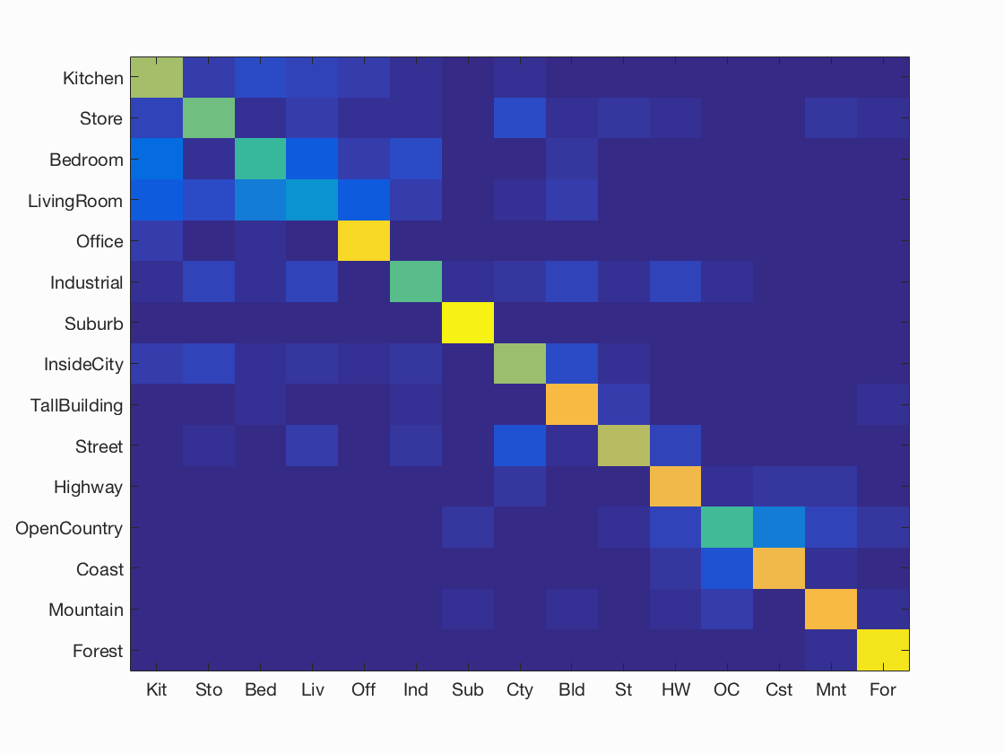
Accuracy (mean of diagonal of confusion matrix) is 0.705
| Category name | Accuracy | Sample training images | Sample true positives | False positives with true label | False negatives with wrong predicted label | ||||
|---|---|---|---|---|---|---|---|---|---|
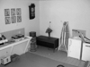
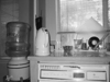
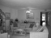
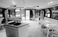
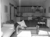
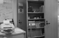
| Kitchen | 0.670 |  |
 |
 |
 |
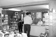 Store |
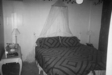
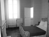 Bedroom |
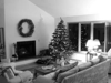
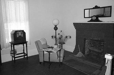
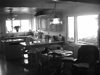 LivingRoom |
 Bedroom |
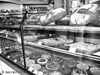
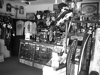
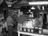
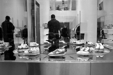
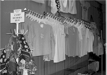
| Store | 0.590 | 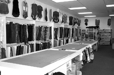 |
 |
 |
 |
 Street |
 Kitchen |
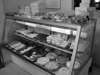 Kitchen |
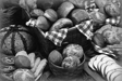 Mountain |
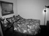
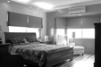
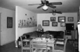
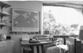
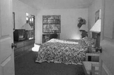
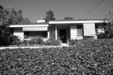
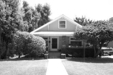
| Bedroom | 0.500 |  |
 |
 |
 |
 Kitchen |
 Kitchen |
 Office |
 Office |
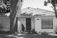
| LivingRoom | 0.310 | 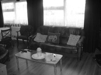 |
 |
 |
 |
 Store |
 Kitchen |
 Kitchen |
 Kitchen |
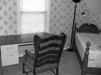
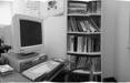
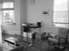
| Office | 0.910 | 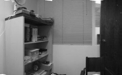 |
 |
 |
 |
 LivingRoom |
 LivingRoom |
 Kitchen |
 Kitchen |
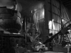
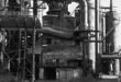
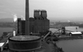
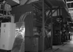
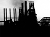
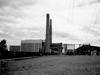
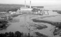
| Industrial | 0.560 |  |
 |
 |
 |
 LivingRoom |
 Bedroom |
 Kitchen |
 OpenCountry |
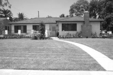
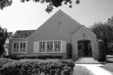
| Suburb | 0.980 | 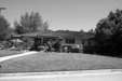 |
 |
 |
 |
 Mountain |
 Highway |
 InsideCity |
 Highway |
| InsideCity | 0.650 |  |
 |
 |
 |
 Street |
 Coast |
 Store |
 TallBuilding |
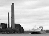
| TallBuilding | 0.820 |  |
 |
 |
 |
 Industrial |
 Industrial |
 Mountain |
 Industrial |
| Street | 0.690 |  |
 |
 |
 |
 TallBuilding |
 Store |
 InsideCity |
 InsideCity |
| Highway | 0.800 |  |
 |
 |
 |
 Industrial |
 Industrial |
 Mountain |
 Store |
| OpenCountry | 0.520 |  |
 |
 |
 |
 Coast |
 Coast |
 Forest |
 Coast |
| Coast | 0.810 |  |
 |
 |
 |
 OpenCountry |
 OpenCountry |
 Highway |
 OpenCountry |
| Mountain | 0.820 |  |
 |
 |
 |
 Highway |
 Highway |
 Forest |
 OpenCountry |
| Forest | 0.950 |  |
 |
 |
 |
 Store |
 Store |
 Store |
 Mountain |
| Category name | Accuracy | Sample training images | Sample true positives | False positives with true label | False negatives with wrong predicted label | ||||