Computer Vision Project

The goal of this project is to examine the task of scene recognition starting with -- tiny images and nearest neighbor classification -- and then move on to more advanced methods -- bags of quantized local features and linear classifiers learned by support vector machines. The basic implementation of this project includes 2 different image representations -- tiny images and bags of SIFT features -- and 2 different classification techniques -- nearest neighbor and linear SVM. In this report, we present performance for the following combinations and extra works.

Part I: Tiny images representation and nearest neighbor classifier

The "tiny image" feature, inspired by the work of the same name by Torralba, Fergus, and Freeman, is one of the simplest possible image representations. One simply resizes each image to a small, fixed resolution (16x16 in this case). It works slightly better if the tiny image is made to have zero mean and unit length. This is not a particularly good representation, because it discards all of the high frequency image content and is not especially invariant to spatial or brightness shifts. We are using tiny images simply as a baseline.

The next task for this part is implementation of nearest neighbor classifier. When tasked with classifying a test feature into a particular category, one simply finds the "nearest" training example (L2 distance is a sufficient metric) and assigns the test case the label of that nearest training example. The nearest neighbor classifier has many desirable features -- it requires no training, it can learn arbitrarily complex decision boundaries, and it trivially supports multiclass problems. It is quite vulnerable to training noise, though, which can be alleviated by voting based on the K nearest neighbors (but you are not required to do so). Nearest neighbor classifiers also suffer as the feature dimensionality increases, because the classifier has no mechanism to learn which dimensions are irrelevant for the decision.

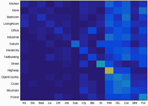
Fig.1: Confusion matrix of tiny image features and nearest neighbor classifier. Click for the more details for the results.

Following code blocks present the tiny image feature and nearest neighbor implementations. The accuracy for tiny image features and nearest neighbor is 20.2%. Figure-1 shows the confusion matrix of the result of this part. Check for the more details for the results.


function image_feats = get_tiny_images(image_paths,img_dim)
if nargin < 2
    img_dim=16;
end
d=img_dim*img_dim;
N=size(image_paths,1);
image_feats=zeros(N,d);

for i=1:N
   I=imread(image_paths{i});
   I=imresize(I,[img_dim img_dim],'bilinear');
   f=reshape(I',[1 d]);
   image_feats(i,:)=f-mean2(f)/std2(f);
end


function predicted_categories = nearest_neighbor_classify (train_image_feats, train_labels, test_image_feats)
N=size(test_image_feats, 1);
predicted_categories = cell(N, 1);
D = vl_alldist2(test_image_feats', train_image_feats');
[~,ind] = min(D,[],2);
for i=1:N
    predicted_categories(i) = train_labels(ind(i));
end

Part II: Bag of SIFT representation and nearest neighbor classifier

Bag of words models are a popular technique for image classification inspired by models used in natural language processing. The model ignores or downplays word arrangement (spatial information in the image) and classifies based on a histogram of the frequency of visual words. The visual word "vocabulary" is established by clustering a large corpus of local features. The step is taken as 16 for this case.

In this part of the project, we move on to a more sophisticated image representation -- bags of quantized SIFT features. Before we can represent our training and testing images as bag of feature histograms, we first need to establish a vocabulary of visual words. We will form this vocabulary by sampling many local features from our training set (10's or 100's of thousands) and then clustering them with kmeans. The number of kmeans clusters is the size of our vocabulary and the size of our features. The step is taken as 8 for this case. Other parameters along with step size are tuned on extra work section.

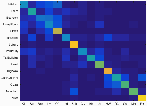
Fig.2: Confusion matrix of bag of SIFT features and nearest neighbor classifier. Click for the more details for the results.

Following code block present bag of SIFT features implementation. The accuracy for bag of SIFT features and nearest neighbor is 53.9%. Figure-2 shows the confusion matrix of the result of this part. Check for the more details for the results.


function image_feats = get_bags_of_sifts(image_paths,step_size)
if nargin < 2
    step_size=8;
end

load('vocab.mat')
vocab_size = size(vocab, 2);
N=size(image_paths,1);
image_feats = zeros(N,vocab_size);
for i=1:N
    I = single(imread(image_paths{i}));
    [~, features] = vl_dsift(I, 'FAST', 'STEP', step_size);
    hist = zeros(1,vocab_size);
    D = vl_alldist2(double(features), double(vocab));
    minD=min(D,[],2);
    for j = 1 : size(D, 1)
        minRow = find(D(j,:) == minD(j));
        hist(minRow) = hist(minRow) + 1;
    end
    hist = double(hist);
    if norm(hist) ~= 0
        hist = hist / norm(hist);
    end
    image_feats(i,:) = hist;
end

Part III: Bag of SIFT representation and linear SVM classifier

In this part, we present how to train 1-vs-all linear SVMS to operate in the bag of SIFT feature space. Linear classifiers are one of the simplest possible learning models. The feature space is partitioned by a learned hyperplane and test cases are categorized based on which side of that hyperplane they fall on. Since linear classifiers are inherently binary, we have a 15-way classification problem. To decide which of 15 categories a test case belongs to, we train 15 binary, 1-vs-all SVMs. Then, all 15 classifiers will be evaluated on each test case and the classifier which is most confidently positive "wins". The free parameter LAMBDA for SVM learning phase has ben set to 0.0001 for now, but it will be tuned in extra credit sections.

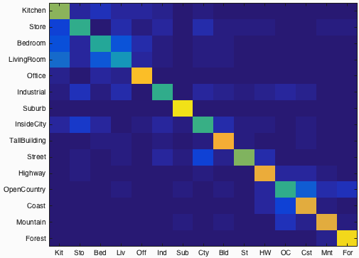
Fig.3: Confusion matrix of bag of SIFT features and linear SVM classifier. Click for the more details for the results.

Following code block present bag of SIFT features implementation. The accuracy for bag of SIFT features and linear SVM classifier is 67.6%. Figure-3 shows the confusion matrix of the result of this part. Check for the more details for the results.


function predicted_categories = svm_classify(train_image_feats, train_labels, test_image_feats,LAMBDA)
if nargin < 4
    LAMBDA=0.0001;
end
categories = unique(train_labels);
num_categories = length(categories);
Ws=[];
Bs=[];

train_size=size(train_image_feats,1);
test_size=size(test_image_feats, 1);
for i = 1 : num_categories
    %Train all images for each category
    category = categories{i};
    category_indices = strcmp(category, train_labels);
    labels = ones(train_size, 1);
    labels(~category_indices) = -1;
    %Train this category now
    [W,B] = vl_svmtrain(train_image_feats', labels, LAMBDA);
    Ws = [Ws; W'];
    Bs = [Bs; B];
end

%Test for all test_image_feats and fill predicted_categories
Bs_size=size(Bs, 1);
predicted_categories=cell(test_size,1);
for i = 1 : test_size
    test_feat = test_image_feats(i, :);
    D = zeros(Bs_size,1);
    for j = 1 : Bs_size
        D(j) = Ws(j, :) * test_feat' + Bs(j);
    end
    maxIndices = find(D == max(D));
    predicted_categories(i) = categories(maxIndices(1));
end

Part IV: Graduate Credit and Extra Work

In this part, we present results of additional works including parameter tunings and improvements for runtime and accuracy.

1- Experiment with features at multiple scales: For this experiment, we perform tiny image representations and nearest neighbor classifier in different scale dimension. To do this, we pick dimensions from 8 to 64 by incrementing it 8 in each iteration and take the running time and accuracies for each. Figure-4 and Figure-5 present the accuracies and running times for each dimension, respectively. The results show that increasing scale size is not a good decision in terms of both for accuracy and efficiency.

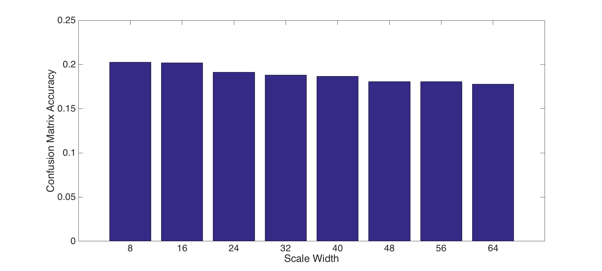
Fig.4: Accuracies for each scale dimension.

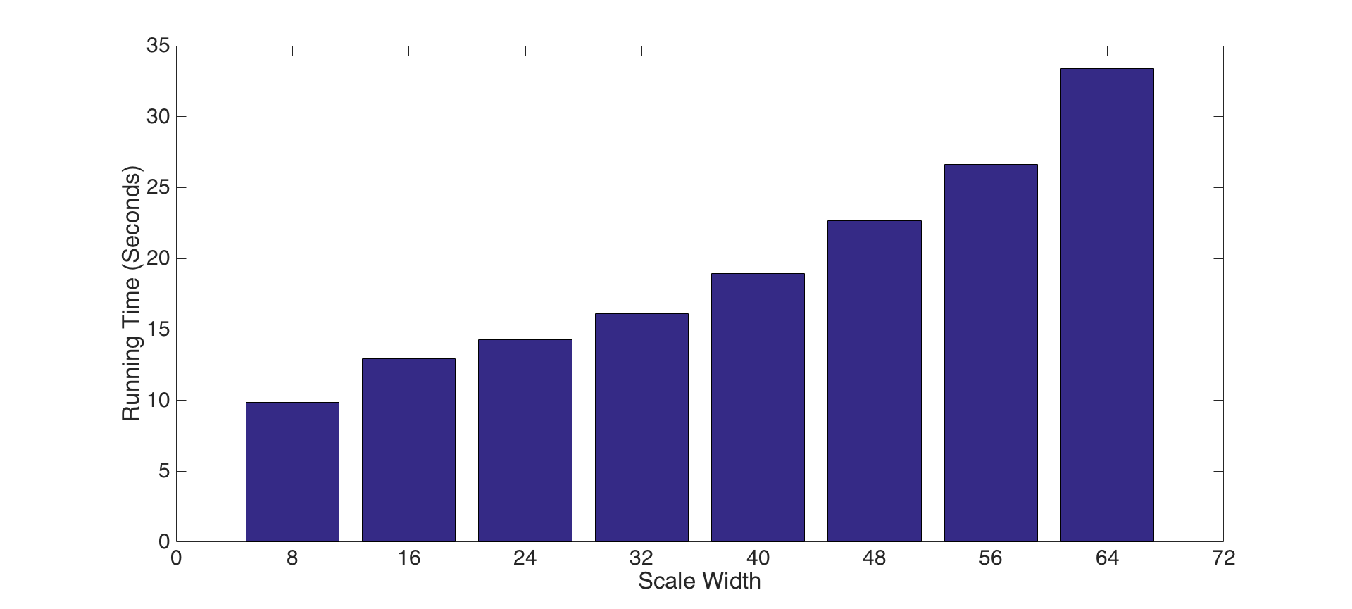
Fig.5: Runtimes for each scale dimension.

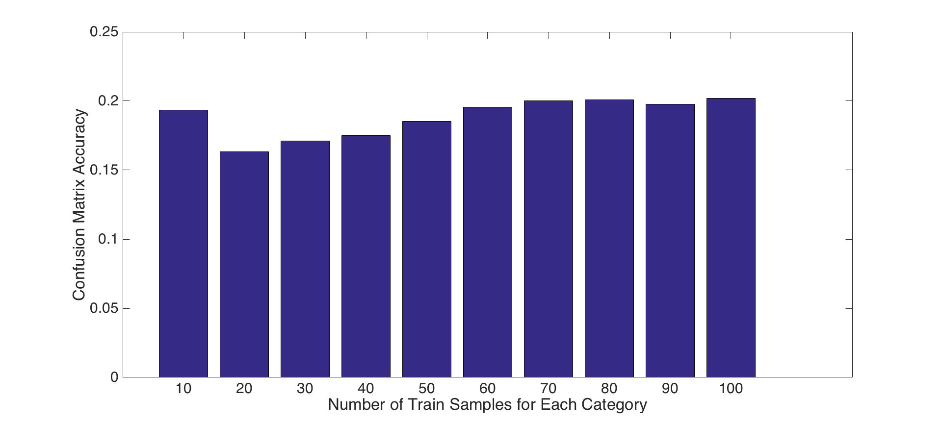
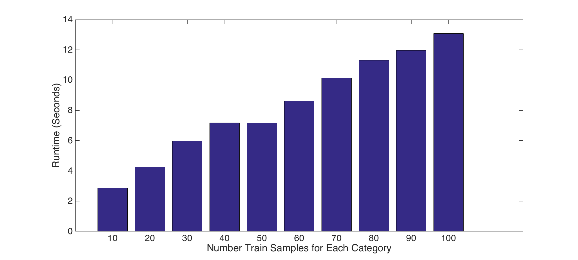
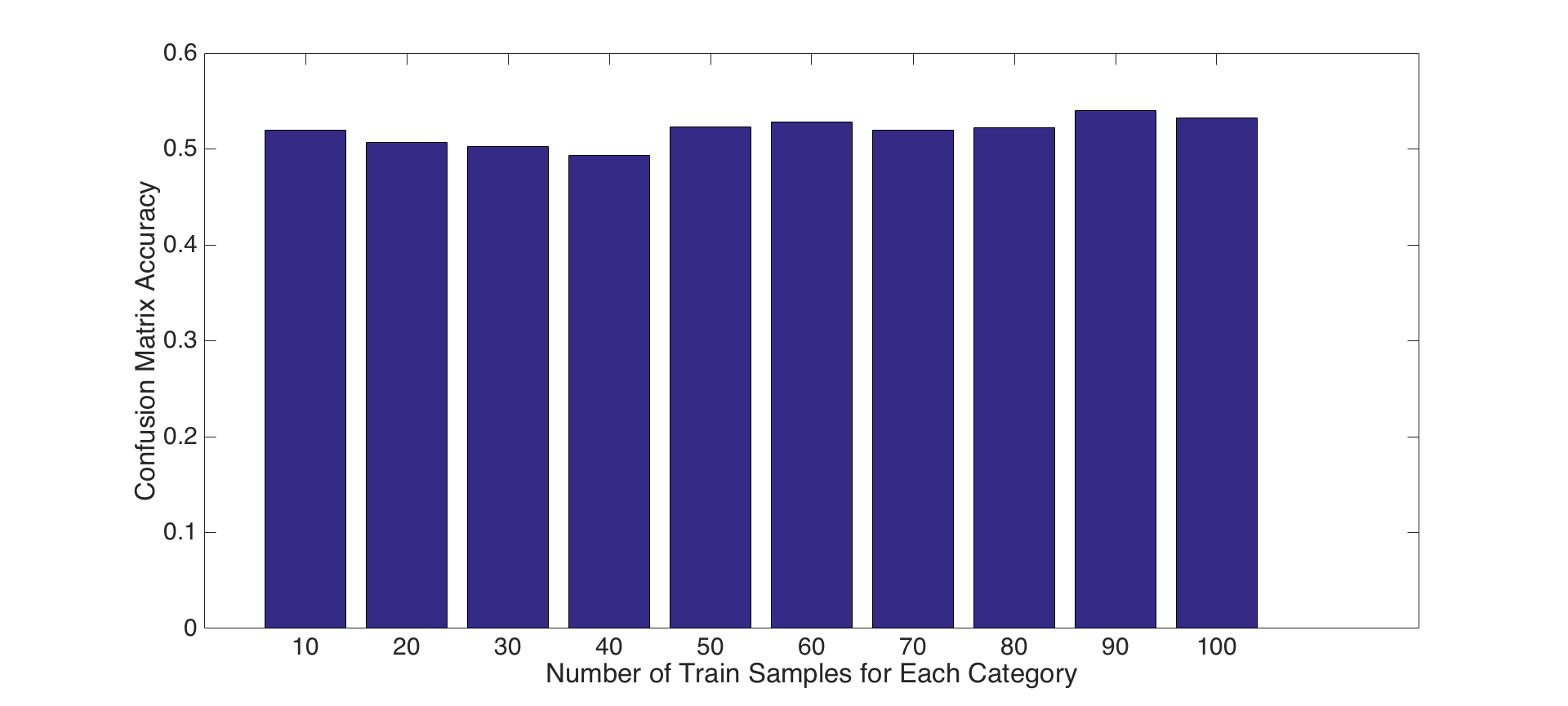
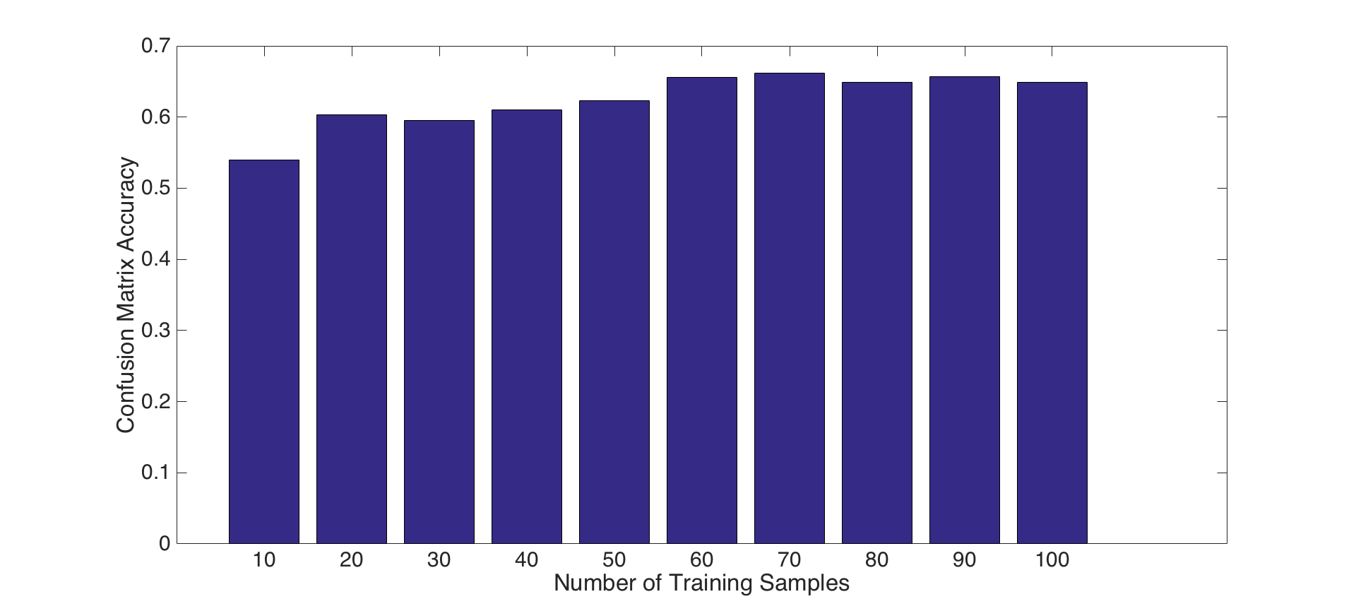
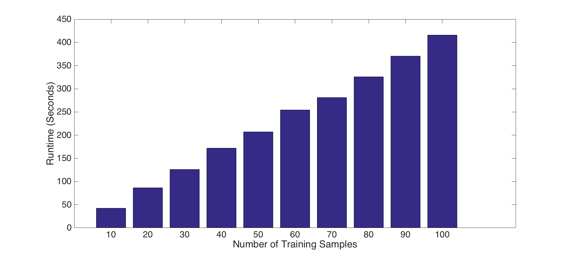
2- Tuning number of training samples parameter: For this experiment, we present the impact of the number of train samples for each parts presented above. To do this, we increment the number of train samples from 10 to 100 by 10 in each iteration, and, repeat this for each feature set and classifier combinations presented above parts. Following figures show the results for accuracy and runtime changes by number of train samples for PART-I, PART-II and PART-III features and classifiers, respectively. Results show that number of train samples how no significant effect on accuracy, but, has negative effect on running time for tiny images and bag of SIFT features with nearest neighbor classifier. That is, accuracies are not increasing as the number of training samples increase, but, running time for training is increasing significantly. Hence, choosing a small number of training samples is a good decision for efficiency. On the other hand, number of training samples has an impact on linear SVM classifier as shown in Figure-8. Although, it increases the running time, it has a reasonable contribution on performance until some points. For instance, after 60 samples the accuracy does not increase too much, but, the running time increase dramatically. Hence using 60-70 samples is a good design decision for both accuracy and efficiency.


Fig.6: Accuracy and Runtime changes by number of train samples for tiny image representations and nearest neighbor classifier.

Fig.7: Accuracy and Runtime changes by number of train samples for bag of SIFT features and nearest neighbor classifier.

Fig.8: Accuracy and Runtime changes by number of train samples for bag of SIFT features and SVM classifier.

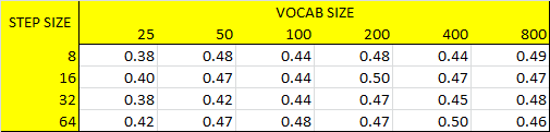
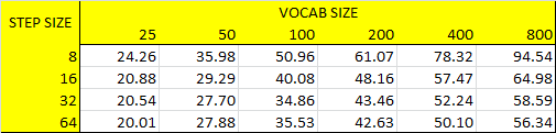
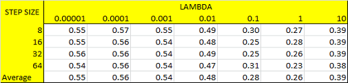
3- Tuning step size, vocab size and LAMBDA values: For this experiment, we present how accuracy and runtime are effected by step size, vocab size and LAMBDA parameters. To do this, we increment LAMBDA values for each vocab size as incrementing vocab size for each step size iteratively. Following code block gives the implementation of this experiment. Following figures show the results for accuracies and runtimes by step size and vocab size for both nearest neighbor and linear SVM classifiers. To make this experiment time efficient, we take the number of training samples as 20 as a result of above experiment. It is worth to note that we pick results for LAMBDA=0.0001 in the following accuracy and runtime figures. Then, we give the average LAMBDA values at each vocab size for each step size in Figure-10 right. Results show that best parameter tuning for both performance and efficiency is achieved by setting step size to 8-16, vocab size to 200-400 and LAMBDA to 0.00001-0.0001. We continue to use vocab size as 200 for efficiency at further analysis.


run('vlfeat/toolbox/vl_setup')
data_path = '../data/';
categories = {'Kitchen', 'Store', 'Bedroom', 'LivingRoom', 'Office', ...
    'Industrial', 'Suburb', 'InsideCity', 'TallBuilding', 'Street', ...
    'Highway', 'OpenCountry', 'Coast', 'Mountain', 'Forest'};
abbr_categories = {'Kit', 'Sto', 'Bed', 'Liv', 'Off', 'Ind', 'Sub', ...
    'Cty', 'Bld', 'St', 'HW', 'OC', 'Cst', 'Mnt', 'For'};

num_train_per_cat = 20;
fprintf('Getting paths and labels for all train and test data\n')
[train_image_paths, test_image_paths, train_labels, test_labels] = ...
    get_image_paths(data_path, categories, num_train_per_cat);


% step_size: 8,16,32,64
% vocab size: 25, 50, 100, 200, 400, 800
% LAMBDA: 0.00001, 0.0001, 0.001, 0.01, 0.1, 1, 10
rt_knn=zeros(4,6);
ac_knn=zeros(4,6);

ac_svm=zeros(4,6,7);

step_size=8;
for i=1:4
    vocab_size=25;
    for j=1:6
        tic
        vocab = build_vocabulary(train_image_paths, vocab_size, step_size);
        save('vocab.mat', 'vocab');
        train_image_feats = get_bags_of_sifts(train_image_paths);
        test_image_feats  = get_bags_of_sifts(test_image_paths);
        predicted_categories = nearest_neighbor_classify(train_image_feats, train_labels, test_image_feats);
        ac_knn(i,j)=create_results_webpage( train_image_paths, test_image_paths, train_labels, test_labels, categories, abbr_categories, predicted_categories);
        rt_knn(i,j)=toc;
        LAMBDA= 0.00001;
        for k=1:7
            predicted_categories = svm_classify(train_image_feats, train_labels, test_image_feats,LAMBDA);
            ac_svm(i,j,k)=create_results_webpage( train_image_paths, test_image_paths, train_labels, test_labels, categories, abbr_categories, predicted_categories);
            LAMBDA=LAMBDA*10;
        end
        vocab_size=vocab_size+25;
        delete vocab.mat
        close all
    end
    step_size=step_size+8;
end


Fig.9: Accuracy rates for each step size by vocab size tuning in both nearest neighbor and linear SVM classifiers (LAMBDA=0.0001 for SVM).

Fig.10: Runtimes for each step size by vocab size tuning on the left. Average LAMBDA values for vocab sizes for each step size on the right.

4- Train the SVM with more sophisticated kernel: For this experiment, we present how accuracy is effected by the choice of SVM kernel. To do this, we used Matlab built-in SVM classification method fitecoc by using different kernel function options such as linear, polynomial and Gaussian/rbf as presented in following code block which resides in svm_kernels.m . We also compare the results with previos section's result that belongs to linear SVM. The accuracies of confusion matrix are 66.69%, 63.80%, 68.50% and 66.90% for vl_svmtrain and Matlab built-in svm classifier with linear, polynomial and rbf kernel functions, respectively. These results show that using polynomial or rbf kernel function has a contribution on the accuracy of classification. Following figures show the confusion matrices of linear, polynomial and rbf kernel functions through left to right.


function predicted_categories = svm_kernels(X, Y, test_image_feats,kernel_function)
% kernel_function={'linear','polynomial','rbf'};
t = templateSVM('KernelFunction',kernel_function);
opt = statset('UseParallel',true);
Mdl = fitcecoc(X,Y,'Coding','onevsall','Learners',t,'Options',opt);
predicted_categories = predict(Mdl,test_image_feats);

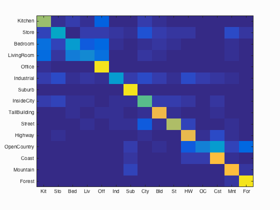
Fig.11: Confusion matrix for linear kernel function. Average accuracy = 63.8%

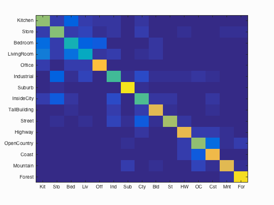
Fig.12: Confusion matrix for polynomial kernel function. Average accuracy = 68.5%

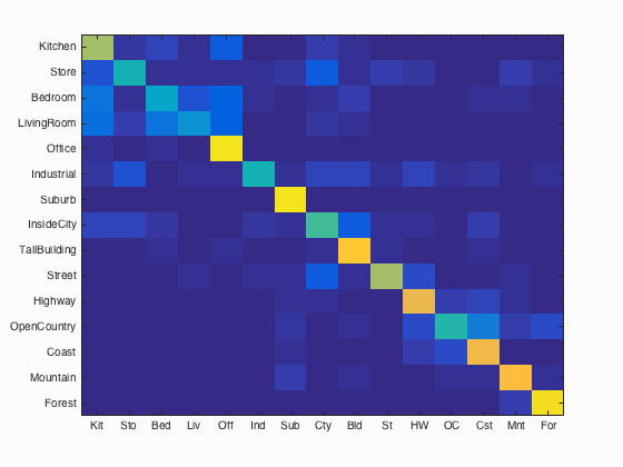
Fig.13: Confusion matrix for Gaussian/rbf kernel function. Average accuracy = 66.9%

5- Add additional, complementary features (Gist Descriptors): For this experiment, we present how accuracy is effected by the additional features. To do this, we include Gist descriptors into our feature base. We use Gist descriptor designed by Aude Oliva and Antonio Torralba. Following code block gives how to call gist descriptor for a single image. We accompany gist descriptor with bag of SIFT features. However, it does not include a significant performance. Confusion matrix below shows an average accuracy of 67.7% for gist descriptor and bag of SIFT features with SVM classifier.

Fig.14: Confusion matrix of bag of SIFT features and Gist descriptor with linear SVM. Accuracy = 67.7%


function gist1=get_gist(img1)
param.imageSize = [256 256]; % it works also with non-square images
param.orientationsPerScale = [8 8 8 8];
param.numberBlocks = 4;
param.fc_prefilt = 4;

[gist1, ~] = LMgist(img1, '', param);
end

Conclusion

Here is our performance evaluation in each step presented above.

Tiny images representation and nearest neighbor classifier = 20.2 %
Bag of SIFT representation and nearest neighbor classifier = 53.9 %
Bag of SIFT representation and linear SVM classifier = 67.6 %
Gist descriptor with bag of SIFT representation and linear SVM classifier = 67.7 %
Bag of SIFT representation and SVM classifier with polynomial kernel function = 68.5 %

Erkam Uzun

Project 4 / Scene Recognition with Bag of Words

Part I: Tiny images representation and nearest neighbor classifier

Part II: Bag of SIFT representation and nearest neighbor classifier

Part III: Bag of SIFT representation and linear SVM classifier

Part IV: Graduate Credit and Extra Work

Conclusion