Project 4 / Scene Recognition with Bag of Words
In this project, our goal is to take an image and classify it into one of 15 categories, ranging from Forests to Offices to Highways. We will be investigating a few different methods of doing this but will ultimately utilize some type of supervised learning.
Random Chance
As is expected, performance from guessing the categories randomly hovers around 6-7% (1 / 15 ~= 0.667).
Tiny Images and KNN
We now employ the strategy of tiny images with k-nearest neighbors. We resize the image to a smaller 16x16 image, adjust the mean of the pixels to 0, and normalize the pixel values to unit length. We will use these normalized pixel values as features and find our nearest neighbors using a mininum L2 distance. A higher value of k means we consider more nearby images. Will this improve performance?
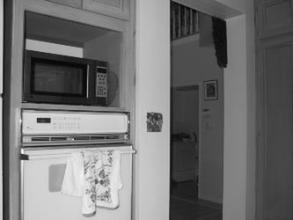
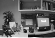
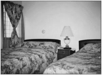
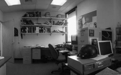
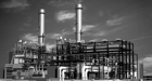
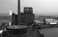
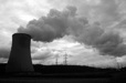
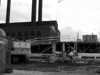
Example large and tiny images side by side (enlarged):

Performance after varying the number of nearest neighbors:
| k | 1 | 5 | 10 | 20 | 30 | 50 | 100 |
| Performance | 22.5% | 21.5% | 21.3% | 22.2% | 21.3% | 20.3% | 19.4% |
As seen above, a larger k does not necessarily mean better performance, at least while using a L2 distance measure. Good performance using knn requires a direct correspondence between the distance measure and the classification categories. Clearly, spatially located pixel intensity is not necessarily a fool-proof indicator of a category placement, although it is easy to imagine that this could work for images where the pixel intensities are correlated (such as a bed being in the middle of the image every time).
Bag of SIFT and KNN
The next step is to use SIFT features as our defining image features. Our procedure is to identify SIFT features for our training images, cluster them with kmeans into a vocabulary of a fixed size, then count how many SIFT features have a closest proximity to each cluster for a given image. We can then use these resulting histograms to classify with k-nearest neighbors. It took a good amount of tweaking to reach a performance of greater than 50%. Notable improvements were increases in knn neighbors (up to a point) and adjustments of SIFT sampling from the images for vocab and training/testing. Below are some of the iterations of tweaking.
| Vocab size | All SIFT width | Vocab SIFT step size | Train/Test SIFT step size | Max # of vocab SIFT features per image | Max # of SIFT features per image | Nearest Neighbors | Performance |
| 200 | 16 | 5 | 5 | 50 | 50 | 1 | 24% |
| 200 | 16 | 50 | 25 | 50 | 300 | 1 | 43.9% |
| 100 | 16 | 15 | 15 | 50 | 500 | 25 | 50.3% |
| 200 | 16 | 22 | 10 | 75 | 250 | 20 | 53.1% |
Scene classification results visualization
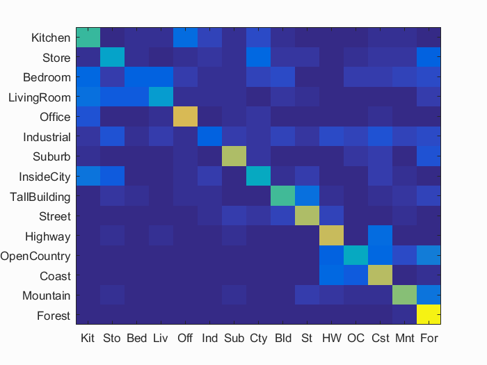
Accuracy (mean of diagonal of confusion matrix) is 0.531
We ultimately ended up with a larger sampling for our vocabulary formation which seemed to be a catalyst for our improvments. Further tweaking would surely improve results even more, but we are now going to move on to our main focus for the assignment.
Bag of SIFT and Support Vector Machine
We now utilize the same SIFT cluster feature histograms as before, except this time we run them through one vs all support vector machines and take the most positive result as our classification. Like the recent methodology, this one took some parameter tuning. First we will briefly discuss our cross validation methodology.
Cross Validation
The regular Performance column below reports the best performance found from running the SVM approximately 5 times. However, a better approach to this is using some type of cross validation. Currently, we use the same train/test split for our training and evaluation. To get a better measure with a single run, I randomly shuffled this split 10 times and reported the average and standard deviation of the overall performances. This was a bit more methodical than the previous method of reporting performance which gives us a more reliable metric.
Now we will move on to the results. One note is about our "features per image" parameter. This parameter samples the SIFT features for an image. The number of SIFT features produced is normally quite high, so we make sure to just get a sampling that is representative of the image to save computation time. Here are just a few of the different parameter runs I performed where I saw leaps in performance:
| Vocab size | All SIFT width | Vocab SIFT step size | Train/Test SIFT step size | Max # of vocab SIFT features per image | Max # of SIFT features per image | SVM Lambda | Performance (best of 5) | Cross Validation (standard deviation) |
| 100 | 8 | 25 | 10 | 100 | 200 | 0.1 | 39.6% | 36.72% (0.02836) |
| 100 | 32 | 40 | 20 | 10 | 50 | 0.1 | 48.1% | 47.5% (0.02220) |
| 200 | 16 | 22 | 10 | 75 | 250 | 0.0002 | 63.0% | 62.7% (0.01365) |
| 10000 | 16 | 22 | 10 | 75 | 250 | 0.0002 | 67.9% | 67.69% (0.01040) |
It became very clear through parameter tweaking that the parameters wildly affected the accuracy of the classification. Performance was very sensitive to the SIFT feature width and SVM lambda, especially. I am confident that there are even better parameter configurations, but I ended up finding the best performance with a SIFT width of 16, a larger vocab size, and a smaller lambda. Early on, it was difficult to determine which parameter was the parameter to change to boost performance. For example, I tested both 8 and 32 SIFT feature widths as seen above. I saw a performance increase with this, but a feature width of 32 ended up taking far too long (~45 minutes vs ~15 minutes). Later, I discovered that a proper small lambda value actually produced significant accuracy boosts to all configurations at the cost of only an extra second or two. The vocab size was also an important performance booster but at the cost of inceased computation time (we will visit this later). The SIFT sample size for the vocab and train/test images actually turned out to be less important than I thought; tweaking these values did not have a huge impact on accuracy or computation time (although of course a very small step size took significantly longer). I still tried to keep with a small sample size for vocab construction and a larger one for train/test features as the vocabulary aims to be a broad sampling of the categories rather than a specific train/test image classification.
Finally, here are our detailed results for the top performing configuration:
Scene classification results visualization
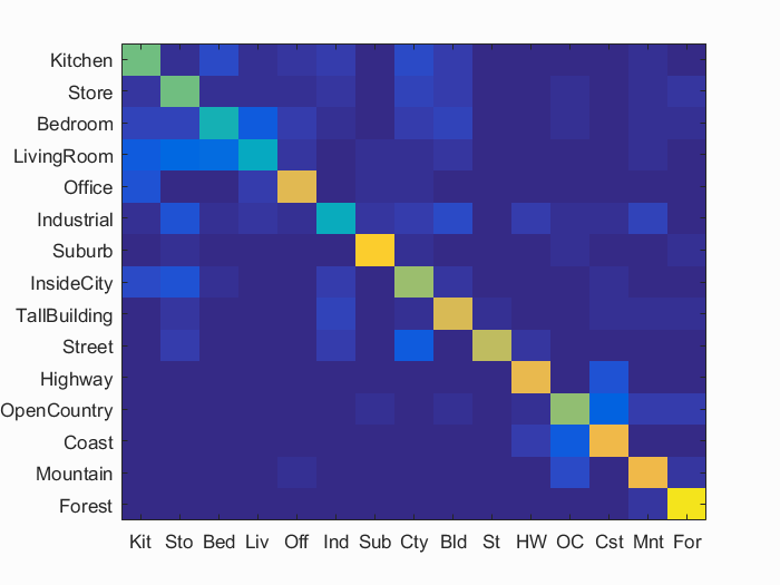
Accuracy (mean of diagonal of confusion matrix) is 0.679
Average cross validation accuracy: 0.6769, standard deviation: 0.01040
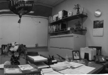
| Category name | Accuracy | Sample training images | Sample true positives | False positives with true label | False negatives with wrong predicted label | ||||
|---|---|---|---|---|---|---|---|---|---|
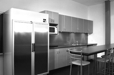
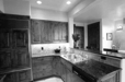
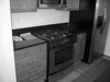
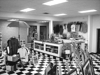
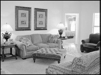
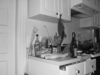
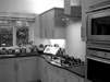
| Kitchen | 0.590 |  |
 |
 |
 |
 Office |
 Office |
 Office |
 LivingRoom |
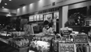
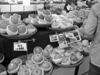
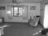
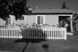
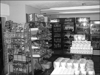
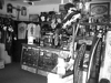
| Store | 0.590 | 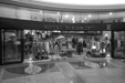 |
 |
 |
 |
 LivingRoom |
 InsideCity |
 OpenCountry |
 Industrial |
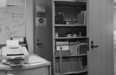
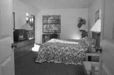
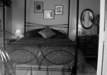
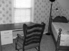
| Bedroom | 0.450 |  |
 |
 |
 |
 LivingRoom |
 LivingRoom |
 TallBuilding |
 TallBuilding |
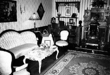
| LivingRoom | 0.400 | 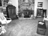 |
 |
 |
 |
 Office |
 Bedroom |
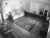 Mountain |
 Kitchen |
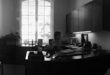
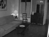
| Office | 0.770 | 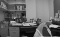 |
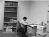 |
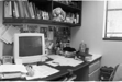 |
 |
 Bedroom |
 Store |
 InsideCity |
 Suburb |
| Industrial | 0.410 |  |
 |
 |
 |
 InsideCity |
 InsideCity |
 Mountain |
 LivingRoom |
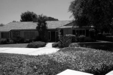
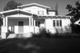
| Suburb | 0.880 | 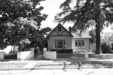 |
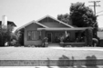 |
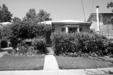 |
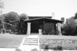 |
 OpenCountry |
 Office |
 Office |
 OpenCountry |
| InsideCity | 0.650 |  |
 |
 |
 |
 Store |
 Suburb |
 Industrial |
 Coast |
| TallBuilding | 0.750 |  |
 |
 |
 |
 Store |
 Kitchen |
 Industrial |
 Industrial |
| Street | 0.710 |  |
 |
 |
 |
 Highway |
 Store |
 InsideCity |
 Highway |
| Highway | 0.790 |  |
 |
 |
 |
 Kitchen |
 OpenCountry |
 Coast |
 Office |
| OpenCountry | 0.640 |  |
 |
 |
 |
 Coast |
 Bedroom |
 Coast |
 Forest |
| Coast | 0.800 |  |
 |
 |
 |
 Industrial |
InsideCity |
 OpenCountry |
 InsideCity |
| Mountain | 0.810 |  |
 |
 |
 |
 Forest |
 Kitchen |
 Forest |
 Office |
| Forest | 0.940 |  |
 |
 |
 |
OpenCountry |
 Mountain |
 Mountain |
 TallBuilding |
| Category name | Accuracy | Sample training images | Sample true positives | False positives with true label | False negatives with wrong predicted label | ||||
It is interesting to consider the higher and lower accuracy categories. The highest accuracy category is the Forest category, at a whopping 94%. This would perhaps suggest that in our SIFT space methodology, an SVM best separates a forest image from other categories. Unfortunately, due to the high dimensionality of both SIFT features and the SVM method, it is difficult to have an easy human intuition to fully explain performance. We might suggest that the shape and distribution of a lot of trees should contribute towards the effective distinction, but we unfortunately do not have the specific understanding of how it actually relates to the implementation. Our lowest performing category is the Living Room category at 40%. It appears that our pipeline is much better at classifying outdoor scenes rather than indoor scenes. My hypothesis is that indoor scenes simply have more complexity: more objects, corners, and general clutter. With this hypothesis, it would make sense that the decision boundaries between these images could be quite populated with ambiguity.
Varying Vocabulary Size
As part of achieving the accuracy above, I wanted to see how the different vocab sizes would affect the performance. A higher vocabulary means more dimensions on the SIFT cluster histograms, allowing for more differentiation between histograms. All runs are identical to the top performing run shown above, apart from the varying vocab sizes. Note that times are rounded to the nearest second. Performance accuracies listed are the maximum accuracies found after 5 runs of the final SVM classification.
| Vocab size | Time to build vocab (seconds) | Time to build train features (seconds) | Time to build test features (seconds) | Performance (best of 5) | Cross Validation (standard deviation) |
| 2 | 453 | 458 | 442 | 16.6% | 16.78% (0.01711) |
| 10 | 458 | 460 | 460 | 41.6% | 41.63% (0.01457) |
| 50 | 487 | 497 | 511 | 58.2% | 56.89% (0.01063) |
| 100 | 488 | 498 | 507 | 60.55% | 60.51% (0.00898) |
| 200 | 457 | 464 | 463 | 63.0% | 62.7% (0.01365) |
| 500 | 501 | 520 | 517 | 64.3% | 64.03% (0.01332) |
| 1000 | 535 | 600 | 619 | 65.6% | 65.49% (0.00534) |
| 5000 | 763 | 1216 | 1226 | 67.4% | 66.88% (0.00894) |
| 10000 | 1023 | 2042 | 2072s | 67.9% | 67.69% (0.01040) |
As seen above, the increased vocabulary size definitely lengthens the process of building the vocabulary and constructing the final histogram of SIFT clusterings. One important design decision is considering this increase in computation time, especially when scaling to many more images in practice. For example, we might be content with a 66% accuracy that completes the pipeline in 25 minutes as opposed to a 67.9% accuracy that completes the pipeline in almost an hour and a half; the diminishing returns are obvious for this parameter.
Getting it under 10 minutes
Most of the results above take at least 20 minutes to run. Can we get a respectable result under 10 minutes?
| Vocab size | SIFT version | All SIFT width | Vocab SIFT step size | Train/Test SIFT step size | Max # of vocab SIFT features per image | Max # of SIFT features per image | SVM Lambda | Time to build vocab (seconds) | Time to build train features (seconds) | Time to build test features (seconds) | Total time | Performance | Cross Validation (standard deviation) |
| 200 | fast | 8 | 85 | 20 | 10 | 100 | .0002 | 25 | 33 | 43 | 1 minute 59 seconds | 56% | 56.28% (0.00908) |
| 200 | fast | 8 | 85 | 20 | 10 | 100 | .0002 | 25 | 33 | 43 | 1 minute 41 seconds | 56% | 56.28% (0.00908) |
| 1000 | fast | 16 | 22 | 10 | 75 | 250 | .0002 | 133 | 176 | 171 | 8 minutes | 66.1% | 65.77% (0.00865) |
| 100 | normal | 4 | 75 | 30 | 10 | 50 | .0002 | 200 | 198 | 186 | 9 minutes 43 seconds | 42.6% | 44.25% (0.00872) |
As shown above, the "fast" SIFT version actually performs very well and much faster than the "full" SIFT method. It manages to rival our best performance number from earlier in much less computation time. The last row shows an attempt to get a "full" SIFT run under 10 minutes by reducing the SIFT feature width, vocab size, and sampling rates. It simply does not compare to performance when using a feature width of 16. It seems that at least for the images we are using, the "fast" SIFT version would be preferred to the "full" version if time is a top concern.
We have seen a few different ways to classify images, and it is easy to see how important it is to experiment with the many free parameters. Machine learning is more of a battle of optimizing the methodology rather than actually choosing the methodology in the first place. In terms of computer vision, we also see how important the makeup of the features are; our use of SIFT and proximity to SIFT clusters histograms proved to be relatively effective.