Project 4 / Scene Recognition with Bag of Words
For this project, 2 different image representations as well as 2 different classifications are implemented. The 2 image representations are tiny images and bags of SIFT features. The 2 classifications are nearest neighbor and SVM. The following 3 combinations of image representations and classfications are completed and compared for results:
- Tiny images and nearest neighbor classifier
- Bag of SIFT features and nearest neighbor classifier
- Bag of SIFT features and linear SVM classifier
Summary:
Tiny Images
Tiny images are obtained literally by resizing each original image into 16x16 squares. The code is shown below:
	size = 16;
	image_feats = zeros([length(image_paths), size*size]);

	for i=1:length(image_paths)
	    img = imread(image_paths{i});
	    img = imresize(img, [size, size], 'bicubic');
	    image_feats(i, :) =  img(:);
	end
Bags of SIFT features
Bags of SIFT features are obtained from building a histogram of existing features(vocab). For each image, the sift features are obtained by using vl_dsift. The distance matrix of SIFT features and vocab is calculated and sorted that the lowest distance for any feature to a vocab is said to correspond to that particular vocab. A histogram counts how many vocab is represented. The code is shown below:
	load('vocab.mat')
	vocab_size = size(vocab, 2);
	N = length(image_paths);
	image_feats = zeros([N, vocab_size]);

	for i=1:N
	    image = imread(image_paths{i});

	    [~, features] = vl_dsift(single(image), 'step', 5);
	    D = vl_alldist2(single(features), vocab);
	    [~, index] = sort(D, 2);

	    hist = zeros([1, vocab_size]);
	    for j=1:size(index, 1)
	        hist(index(j, 1)) = hist(index(j, 1)) + 1;
	    end
	    hist = hist ./ norm(hist);
	    image_feats(i, :) = hist;
	end
A step size of 5 for vl_dsift is chosen for performance/speed trade off.
Nearest Neighbor Classifier
Nearest neighbor classifier works by calculating distances between test image features and train image features. The distance matrix is sorted so that the lowest distance index is on the first column. The index is then turned into labels for each image. The code is shown below:
	D = vl_alldist2(test_image_feats', train_image_feats');
	[~, index] = sort(D, 2);

	predicted_categories = train_labels(index(:,1), :);
SVM Classifier
15 classifiers for built. One for each unique category in the labels. For each category, the labels for all training images are turned into -1 and 1 for positive and negative. A SVM classifier is trained using the new labels. Using the classifier, test images obtain either positive or negative values where positive value indicates a potential true and negative value indicates a potential false. The magnitude of the values indicate the confidence of the classifier. The results for all images are stored and sorted so that the highest value index is converted into a text label that represents the category for images. The code is shown below:
	categories = unique(train_labels);
	num_categories = length(categories);
	M = size(test_image_feats, 1);
	LAMBDA = 0.000049;
	results = zeros([num_categories, M]);
	for i=1:num_categories
	     matching_indices = strcmp(categories{i}, train_labels);
	     labels = zeros(length(train_labels), 1);
	     for j=1:length(matching_indices)
	        if(matching_indices(j) == 1)
	            labels(j) = 1;
	        else
	            labels(j) = -1;
	        end
	     end
	    [W, B] = vl_svmtrain(train_image_feats', labels, LAMBDA);
	    results(i, :) = W' * test_image_feats' + B;
	end

	[~, index] = sort(results, 1, 'descend');
	predicted_categories = categories(index(1, :));
Different lambda between 0.01 and 0.00001 are tried. It is obvious that some value in between the two will produce a best performing lambda, thus a binary search is used with everything else constant.
Results without time constraints
- Tiny images and nearest neighbor classifier: 19.1%
- Bag of SIFT features and nearest neighbor classifier: 54.1%
- Bag of SIFT features and linear SVM classifier: 69.3%
Results with time constraints
- Tiny images and nearest neighbor classifier: 19.1% Run time: 00:08
- Bag of SIFT features and nearest neighbor classifier: 51.2% Run time: 02:39
- Bag of SIFT features and linear SVM classifier: 63.4% Run time: 02:44
Best Result
Best result comes from the implementation of
Scene classification results visualization
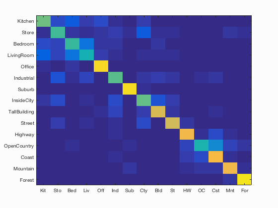
Accuracy (mean of diagonal of confusion matrix) is 0.693
| Category name | Accuracy | Sample training images | Sample true positives | False positives with true label | False negatives with wrong predicted label | ||||
|---|---|---|---|---|---|---|---|---|---|
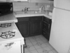
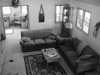
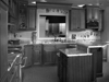
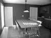
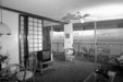
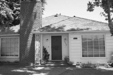
| Kitchen | 0.580 |  |
 |
 |
 |
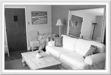
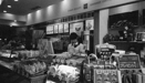
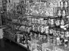
 Store |
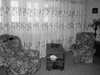
 LivingRoom |
 LivingRoom |
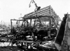
 Industrial |
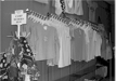
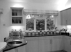
| Store | 0.530 | 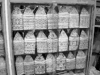 |
 |
 |
 |
 InsideCity |
 Forest |
 Street |
 Forest |
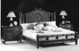
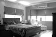
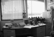
| Bedroom | 0.510 |  |
 |
 |
 |
 Kitchen |
 Kitchen |
 Store |
 LivingRoom |
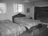
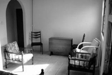
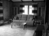
| LivingRoom | 0.450 |  |
 |
 |
 |
 Industrial |
 Bedroom |
 Kitchen |
 Office |
| Office | 0.910 |  |
 |
 |
 |
 Bedroom |
 LivingRoom |
 Bedroom |
 Street |
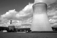
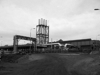
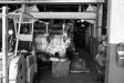
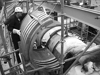
| Industrial | 0.560 |  |
 |
 |
 |
 InsideCity |
 Store |
 OpenCountry |
 LivingRoom |
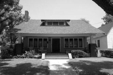
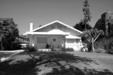
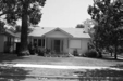
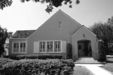
| Suburb | 0.930 | 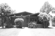 |
 |
 |
 |
 OpenCountry |
 Mountain |
 Industrial |
 InsideCity |
| InsideCity | 0.570 |  |
 |
 |
 |
 Industrial |
 LivingRoom |
 Street |
 Industrial |
| TallBuilding | 0.760 |  |
 |
 |
 |
 InsideCity |
 LivingRoom |
 Industrial |
 Industrial |
| Street | 0.740 |  |
 |
 |
 |
 TallBuilding |
 Industrial |
 Highway |
 InsideCity |
| Highway | 0.810 |  |
 |
 |
 |
 Coast |
 Street |
 Mountain |
 Coast |
| OpenCountry | 0.460 |  |
 |
 |
 |
 Highway |
Industrial |
 Highway |
 Coast |
| Coast | 0.820 |  |
 |
 |
 |
 OpenCountry |
 Highway |
 OpenCountry |
 OpenCountry |
| Mountain | 0.810 |  |
 |
 |
 |
 Forest |
 Industrial |
Suburb |
 Highway |
| Forest | 0.950 |  |
 |
 |
 |
 Store |
 Store |
 Mountain |
 Mountain |
| Category name | Accuracy | Sample training images | Sample true positives | False positives with true label | False negatives with wrong predicted label | ||||
It can be seen that this SVM and bags of SIFT features combinations works the best with forest and mountain categories. It is undestood since those landscapes usually possess lots of unqiue identifing combinations of features.