Project 4 / Scene Recognition with Bag of Words
Overview
For this project, a 15 scene dataset was classified using combinations of three types of features and two types of classifiers. The features used were tiny images, bag of SIFT, and Fisher encoding. For classification, 1-Nearest Neighbor (1NN) and one-vs-all linear Support Vector Machines (SVM) were tested with these different features. Each of the parameters (including SIFT step size, SVM lambda, and vocab size) was tuned using a validation set before running on the test set. The results showed that the Fisher encoding with SVM produced the highest average class accuracy at 78.2%.
Feature Extraction
The first stage of the scene recognition pipeline involved computing a set of features for each of the training images to be fed into the classifier. The following sections describe each of the methods used and their Matlab implementations.
Tiny Images
The tiny image feature is a very simple feature created by resizing each image to a much smaller resolution. Shown below is the Matlab implementation of this feature in the get_tiny_images() function:
% Load and resize images
imsize = 16;
image_feats = zeros(size(image_paths, 1), imsize^2);
for i = 1:size(image_paths,1)
    im = imread(image_paths{i});
    image_feats(i,:) = reshape(imresize(im, [imsize, imsize]), 1, imsize^2);
end

% Normalize to zero mean, unit length
image_feats = bsxfun(@minus, image_feats, mean(image_feats, 2));
image_feats = bsxfun(@times, image_feats, 1./sqrt(sum(image_feats.^2, 2)));
This code begins by defining the image size. In this case, a 16x16px size was used. For each of the input images, the imresize() Matlab function scales down the image, which is then flattened into a single feature vector. To improve performance, the tiny images are also normalized to zero mean and unit length.
Bag of SIFT
For the bag of SIFT feature, the first step is to create a vocabulary of SIFT features sampled from the training images. This is done in the build_vocabulary() function below:
% SIFT step size
STEP_SIZE = 75;

% Get SIFT features from training images
features = cell(1, size(image_paths, 1));
for i = 1:size(image_paths, 1)
    [~, features{1,i}] = vl_dsift(single(imread(image_paths{i})), 'Step', STEP_SIZE, 'Fast');
end

% Cluster the SIFT features to create a vocabulary
[centers, ~] = vl_kmeans(single(cell2mat(features)), vocab_size);
vocab = centers';
The beginning of this function declares the step size at which the SIFT features are computed. The step size used was 75, which was tuned using a validation set (see Results section below). For each training image, a set of SIFT features was computed. The SIFT algorithm was run using the "Fast" parameter because this caused a significant speedup in computation time and was found to have little effect on the final results. After the SIFT features were computed, they were clustered using K-Means. The vocabulary size used was 200, which was also tuned using the validation set (see Results section).
After the vocabulary was computed, the bag of SIFT features for each image were found using the Matlab function get_bags_of_sift(), shown below:
% Load in precomputed vocabulary
load('vocab.mat')
vocab_size = size(vocab, 2);

% SIFT step size
STEP_SIZE = 5;

image_feats = zeros(size(image_paths, 1), vocab_size);
for i = 1:size(image_paths, 1)
    % For each image, get SIFT features
    [~, features] = vl_dsift(single(imread(image_paths{i})), 'Step', STEP_SIZE, 'Fast');

    % Compare distance between each of the image's SIFT features and vocab
    D = vl_alldist2(single(features), vocab');

    % Create normalized histogram over minimum distance cluster centers
    [~, inds] = min(D, [], 2);
    [image_feats(i,:), ~] = histcounts(inds, 1:vocab_size+1, 'Normalization', 'probability');
end
This function loads the precomputed vocabulary and declares the SIFT step size. This step size was chosen to be smaller than the size used for computing the vocabulary to produce more features. The step size chosen was 5, which was determined using a validation set (see Results section). For each image, the SIFT features were computed at this step size. The "Fast" parameter was used here in addition to the vocabulary computation because of the significant speedup and minimal effect on the results. For each of the SIFT features, the distance between the feature and each vocabulary word was computed. The minimum distance vocab word was taken for each feature, and a histogram over these minimum distance vocabulary words was used as the feature encoding for each image. The histogram was also normalized as a probability since it is possible that not all images will have the same number of SIFT features.
Fisher Encoding (Extra Credit)
The final feature extraction method used was the Fisher encoding, described in Chatfield et al. and Perronnin et al. This method is similar to the bag of SIFT feature, but uses a Gaussian Mixture Model (GMM) instead of the K-means clustering and the Fisher encoding rather than a histogram count. The vocabulary creation code for the Fisher encoding was implemented in the build_fisher_vocab() function below:
% SIFT step size
STEP_SIZE = 75;

% Get SIFT features for each image
features = cell(1, size(image_paths, 1));
for i = 1:size(image_paths, 1)
    [~, features{1,i}] = vl_dsift(single(imread(image_paths{i})), 'Step', STEP_SIZE, 'Fast');
end

% Use GMM as vocabulary
[means, covariances, priors] = vl_gmm(single(cell2mat(features)), vocab_size);
The Fisher vocabulary begins with the same step size and SIFT feature extraction as the build_vocab() function. However, instead of K-Means, it computes the means, covariances, and priors of a GMM with the specified vocabulary size (200). Instead of storing the cluster centers, this code will store the means, covariances, and priors which will be used as input to the Fisher encoding algorithm.
After the vocabulary is generated, the Fisher encoding for each image is computed using the function get_fisher_enc() below:
% Load vocabulary
load('fisher_vocab.mat')
vocab_size = size(means, 2);

% SIFT step size
STEP_SIZE = 5;

image_feats = zeros(size(image_paths, 1), 2*vocab_size*128);
for i = 1:size(image_paths, 1)
    % For each image, get SIFT features with smaller step size
    [~, features] = vl_dsift(single(imread(image_paths{i})), 'Step', STEP_SIZE, 'Fast');
    image_feats(i,:) = vl_fisher(single(features), means, covariances, priors);
end
The first lines in this function load the previously generated means, covariances, and priors from the GMM. The SIFT step size is kept the same as the get_bags_of_sift() step size. For each image, the SIFT features are calculated, and VLFeat's vl_fisher() function performs the Fisher encoding on these SIFT features. The Fisher encoding is used as input to the classification stage in place of the histogram count used in the bag of SIFT.
Classification
For the classification stage of the scene recognition pipeline, two classification algorithms, including 1NN and SVM, were implemented in Matlab. The following sections describe the implementations for each of the algorithms.
1NN
For the 1NN classifier, each input point was assigned the same class label as the single nearest neighboring training point. This was done using the Matlab function nearest_neighbor_classify():
% Find distance between each test image and each train image
D = vl_alldist2(train_image_feats', test_image_feats', metric);

% Take the min distance for each test image
[~, I] = min(D);

% Get label of closest training point
predicted_categories = train_labels(I);
This code first computes the distance between each training and test point. The distance metric that produced the best results for the tiny images set was the L2 distance, and the CHI2 distance metric yielded the best results for the bag of SIFT features. After the distances are computed, the minimum distance training point is found for each test point and the corresponding label from the training point is taken as the predicted test label.
SVM
In addition to the 1NN classifier, a one-vs-all linear SVM classifier was implemented in Matlab using the svm_classify() function below:
categories = unique(train_labels);
num_categories = length(categories);
lambda = 0.00001;

% Train SVM classifiers
confidences = ones(size(test_image_feats, 1), 1) * -inf;
predicted_categories = cell(size(test_image_feats, 1), 1);
for i = 1:num_categories
    % Train classifier for this category vs rest
    labels = strcmp(categories(i), train_labels) * 2 - 1;
    [W, B] = vl_svmtrain(train_image_feats', labels, lambda);

    % Get test results for this classifier
    test_results = W' * test_image_feats' + B;

    % Save confidence and predicted category if greater than current confidence
    idx = test_results' > confidences;
    confidences(idx) = test_results(idx');
    predicted_categories(idx) = categories(i);
end))
The first part of this code defines the categories as well as the lambda parameter. This parameter was tuned to 0.00001 using a validation set (see Results section). Next, the code creates an SVM for each category and trains on that category versus all of the remaining categories. It then feeds the test data through each of the classifiers and finds the classifier with the highest confidence for each data point. The label corresponding to the most confident SVM classifier is then assigned to the test point.
Results
The following sections show the accuracy on the validation set for different parameters as well as the accuracy on the full test set compared for each combination of feature extraction and classification algorithms.
Parameter Tuning with Validation Set (Extra Credit)
In order to tune each of the parameters in the feature extraction and classification algorithms, a validation set was created by dividing the training set in half. Examples from each class were divided evenly between the training and validation sets. The first set of parameters tuned using the validation set were the SIFT step sizes used for computing the vocabulary and extracting the features. These two parameters were tuned using the Fisher encoding with SVM. The vocab size was fixed to a value of 200 and the SVM lambda value was fixed at 0.0001 when tuning the step sizes. The following table shows the validation accuracy for different combinations of the two step sizes:
| Vocab Step Size | Feature Step Size | Validation Accuracy (%) |
| 25 | 5 | 67.7 |
| 25 | 10 | 59.7 |
| 25 | 15 | 53.1 |
| 50 | 5 | 68.3 |
| 50 | 10 | 60.5 |
| 50 | 15 | 54.0 |
| 75 | 5 | 71.2 |
| 75 | 10 | 62.9 |
| 75 | 15 | 57.7 |
| 100 | 5 | 69.9 |
| 100 | 10 | 64.7 |
| 100 | 15 | 58.7 |
The validation results show that the highest accuracy was achieved for a vocabulary step size of 75 and a feature extraction step size of 5, with an accuracy of 71.2%. These two step sizes were then fixed and the SVM lambda value was tuned with the validation set. Since the Fisher encoding showed only very small differences in accuracy across lambda values, the bag of SIFT feature was used instead for tuning lambda. The validation results for different lambdas are shown in the table below:
| Lambda | Validation Accuracy (%) |
| 0.001 | 41.1 |
| 0.0001 | 54.0 |
| 0.00001 | 58.5 |
| 0.000001 | 56.5 |
| 0.0000001 | 50.9 |
A lambda value of 0.00001 yielded the highest validation accuracy for bag of SIFT features at 58.5%, so this value was selected as the final lambda value.
Selecting a Vocab Size (Extra Credit)
After determining the best parameters for each of the algorithms, the validation set was used to test the accuracy across different vocabulary sizes. The validation accuracy was computed using Fisher encoding with SVM with the parameters from the previous section. The results of the analysis are found in the following table:
| Vocab Size | Validation Accuracy (%) |
| 10 | 58.1 |
| 20 | 64.8 |
| 50 | 67.9 |
| 100 | 69.1 |
| 200 | 71.2 |
| 400 | 68.3 |
| 1000 | 67.6 |
The vocabulary size that produced the best results was 200. Larger vocabulary sizes resulted in slight performance decreases (likely from overfitting) in addition to very slow computation time.
Method Comparison
After selecting the best parameters for each method using the validation set, each of the recognition pipelines was run on the test set. The four pipelines used were tiny images with 1NN, bag of SIFT with 1NN, bag of SIFT with SVM, and Fisher encoding with SVM. The resulting accuracies for these pipelines are shown in the table below:
| Feature | Classifier | Test Accuracy (%) |
| Tiny Images | 1NN | 22.5 |
| Bag of SIFT | 1NN | 55.9 |
| Bag of SIFT | SVM | 63.1 |
| Fisher Encoding | SVM | 78.2 |
The weakest recognition accuracy was achieved with the tiny images feature. This feature is overly simplistic, and not very descriptive, so the accuracy was not very strong at 22.5%. Using bag of SIFT features with 1NN more than doubled this accuracy to 55.9% since the bag of SIFT features are more informative. However, the 1NN algorithm limited this performance because of its sensitivity to noise by only selecting the single nearest training image. Switching to a one-vs-all linear SVM increased accuracy with bag of SIFT by 7.2% to an accuracy of 63.1%. The highest accuracy was achieved using the Fisher encoding with the SVM. This approach significantly increased the accuracy to 78.2%. The confusion matrix for the Fisher encoding and SVM approach is shown below, along with several positive and negative classification examples:
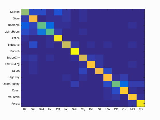
Accuracy (mean of diagonal of confusion matrix) is 0.782
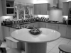
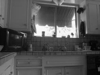
| Category name | Accuracy | Sample training images | Sample true positives | False positives with true label | False negatives with wrong predicted label | ||||
|---|---|---|---|---|---|---|---|---|---|
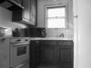
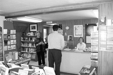
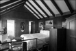
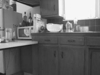
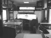
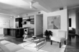
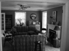
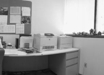
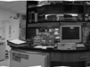
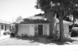
| Kitchen | 0.630 | 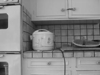 |
 |
 |
 |
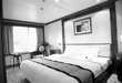
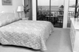
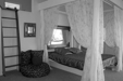
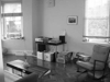
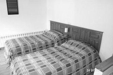
 Bedroom |
 Office |
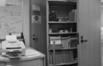
 Office |
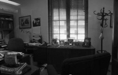
 Office |
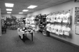
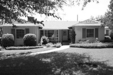
| Store | 0.820 |  |
 |
 |
 |
 TallBuilding |
 InsideCity |
 Kitchen |
 Kitchen |
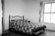
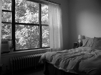
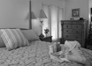
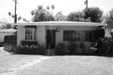
| Bedroom | 0.570 | 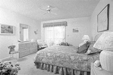 |
 |
 |
 |
 LivingRoom |
 Kitchen |
 Kitchen |
 Kitchen |
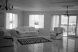
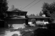
| LivingRoom | 0.560 | 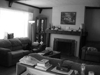 |
 |
 |
 |
 Bedroom |
 Bedroom |
 Bedroom |
 Kitchen |
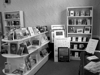
Office | 0.940 | 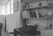 |
 |
 |
 |
 LivingRoom |
 LivingRoom |
 Kitchen |
 LivingRoom |
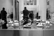
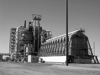
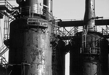
| Industrial | 0.730 | 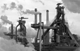 |
 |
 |
 |
 Store |
 Bedroom |
 LivingRoom |
 LivingRoom |
| Suburb | 0.990 | 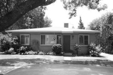 |
 |
 |
 |
 OpenCountry |
 InsideCity |
 TallBuilding |
|
| InsideCity | 0.760 |  |
 |
 |
 |
 Highway |
 Street |
 TallBuilding |
 LivingRoom |
| TallBuilding | 0.850 |  |
 |
 |
 |
 Industrial |
 Store |
 Bedroom |
| Street | 0.800 |  |
 |
 |
 |
 InsideCity |
 Mountain |
 Store |
 Industrial |
| Highway | 0.830 |  |
 |
 |
 |
 OpenCountry |
 Street |
 InsideCity |
 Coast |
| OpenCountry | 0.580 |  |
 |
 |
 |
 Highway |
 Coast |
 Mountain |
 Coast |
| Coast | 0.860 |  |
 |
 |
 |
 OpenCountry |
 OpenCountry |
 Highway |
 OpenCountry |
| Mountain | 0.860 |  |
 |
 |
 |
 Bedroom |
 TallBuilding |
 OpenCountry |
 Highway |
| Forest | 0.950 |  |
 |
 |
 |
 TallBuilding |
 Mountain |
 Mountain |
 Street |
| Category name | Accuracy | Sample training images | Sample true positives | False positives with true label | False negatives with wrong predicted label | ||||
The Fisher encoding and SVM method had the highest accuracies for the suburb (99%) and forest (95%) classes. These two classes are generally quite distinct from the other classes, which may have contributed to their high accuracies. The lowest accuracies occurred with the living room (56%) and bedroom (57%) classes. These two scenes often look alike, so the classifier tended to misclassify one as the other quite often.
Fast Computation
To reduce the computation time of the bag of SIFT feature to under 10 minutes, the step size can be increased to 10. This results in the following accuracies for each of the two classifiers:
| Method | Accuracy (%) |
| Bag of SIFT 1NN | 51.7 |
| Bag of SIFT SVM | 59.9 |