Project 4 / Scene Recognition with Bag of Words
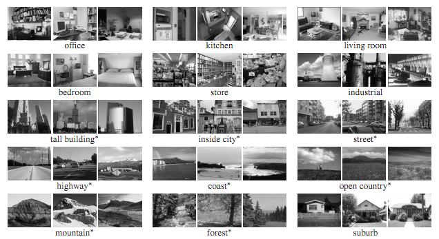
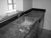
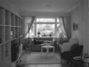
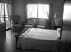
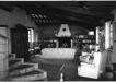
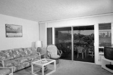
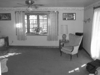
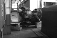
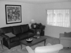
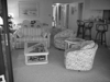
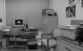
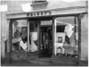
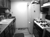
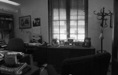
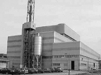
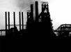
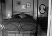
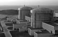
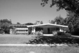
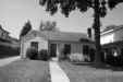
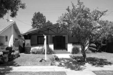
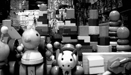
Sample images from categories
One of the fundamental problems that computer vision aims to solve is the ability to recognize objects and scenes in images. The idea is simple: given an image of a scene, return a meaningful value as to what that scene represents. As this problem is widely researched, many useful algorithms have been developed to aid in this task. This project aims to look at some of the methods used over the years to identify images within the 15 scene database as described in Lazebnik et al. 2006 . This database consists of 15 different scenes including: forest, kitchen, industrial, mountain, coast, and others. In each scene are 100 images, each with a correct label. The goal is to acheive 70% accuracy for all 1500 images.
Approaches
This project attempts 3 different approaches to identify a scene within an image.
- Tiny Images with Nearest Neighbor Classifier
- Bag of SIFTs with Nearest Neighbor Classifier
- Bag of SIFTs with SVM Classifier
Feature Representation
Tiny Images
Tiny Images is the simplest form of image representation. Input an image and output the same image, just scaled down to some fixed length. You lose a lot of information through this process, and it will change with differences in color or brightness, but it is simple to implement as shown here:
    result = zeros(size(image_paths, 1), 256);

    for i=1:size(image_paths,1)
        img = imread(image_paths{i});
        resized = imresize(img, [16 16]);
        result(i, :) = resized(:);
    end

    image_feats = result;
Tiny Images along with the Nearest Neighbor classify acheived an accuracy of 20.5%.
Bag of SIFT
Like in project 2, SIFT features are not overly complicated ways of describing images using histograms of gradients. The Bag of SIFT features takes these one step further. Using training images, a vocabulary of SIFT descriptors is built. Then for each image, more SIFT features are found and each one is matched to its nearest SIFT feature in the vocabulary. Then, much like in the SIFT feature itself, a histogram is built consisting of what vocabulary SIFT features were found in each image. Let's look at what one of the histograms can actually look like.
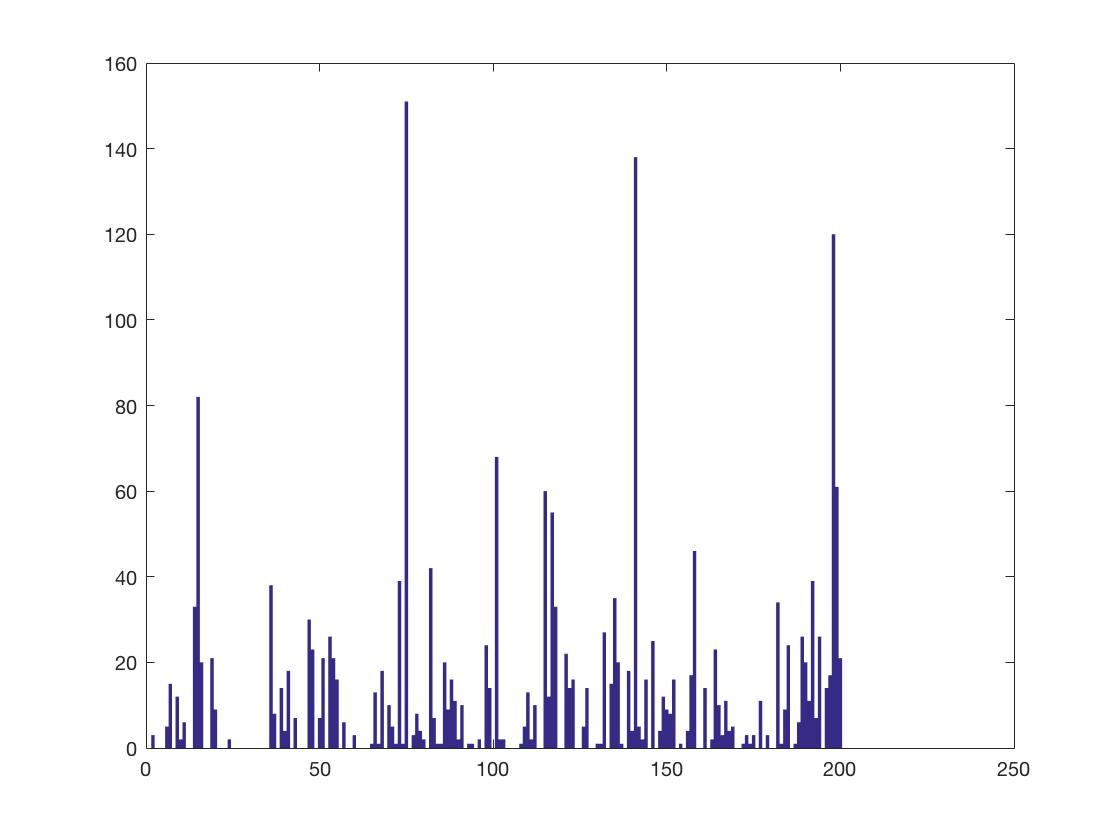
Looking at the histogram, the most common vocabulary SIFT examples were found at around SIFT #75, SIFT #140, and SIFT #200. Thus, images that had similar results would be classified as the same scene.
Now knowing what these features look like, the code to create these features looks like this:
    BAGS_STEP_SIZE = 5;
    BIN_SIZE = 8;

    result = zeros(size(image_paths, 1), vocab_size);

    for i=1:size(image_paths, 1)
        % compute sift features
        img = imread(image_paths{i});
        [locations, SIFT] = vl_dsift(single(img),...
            'fast',...
            'step', BAGS_STEP_SIZE,...
            'size', BIN_SIZE);

        % match to closest cluster
        distances = vl_alldist2(double(SIFT), vocab');
        [matches, indicies] = min(distances');

        % compute histogram
        histogram = zeros(1, vocab_size);
        for j=1:size(indicies,2)
            histogram(indicies(j)) = histogram(indicies(j)) + 1;
        end

        % assign histogram to image_feats(i, :)
        result(i, :) = normr(histogram);
    end

    image_feats = result;
Classifier
Nearest Neighbor
Nearest Neighbor matching is a fast and easy method of classification that produces decent accuracies. The idea is to calculate the distance to each feature's cluster center, and simply choose the closest one. Code for this method can be seen here:
    distances = vl_alldist2(test_image_feats', train_image_feats', 'chi2')';
    [mins, indicies] = min(distances, [], 2);
    predicted_categories = train_labels(indicies);
Using Bag of SIFT and Nearest Neighbor Classification, achieved an accuracy of 52.0%.
SVM
Nearest neighbor works decently, but accuracies could be improved through the next iteration of the project by using a SVM Machine. An SVM Machine, however, makes binary decisions. It can be trained to classify an image as either a forest scene, or not a forest scene. Decisions need to be made for 15 scene categories though, so 15 different SVM Machine's need to be created. Each image is then run through every single classifier and whichever one outputs the highest confidence in its decision will be the final scene decision. The code using SVM Machine classification can be seen here:
    categories = unique(train_labels);
    num_categories = length(categories);
    LAMBDA = 10;

    ws = zeros(15, size(train_image_feats, 2));
    bs = zeros(15, 1);

    for i=1:num_categories
        category = categories(i);
        binary = double(strcmp(category, train_labels));
        binary(binary == 0) = -1;
        [W B] = vl_svmtrain(train_image_feats', binary, LAMBDA);
        ws(i, :) = W;
        bs(i, :) = B;
    end

    result = train_labels;

    for i=1:size(test_image_feats, 1)
        confidences = dot(ws,...
            repmat(test_image_feats(i, :), num_categories, 1),...
            2) + bs;
        [match, index] = max(confidences);
        result(i) = categories(index);
    end

    predicted_categories = result;
Bag of SIFT features and an SVM classifer achieved an accuracy of 65.97%.
Parameter Values
Step Size
The step size is an important parameter in two locations. In building the vocabulary, the step size was chosen to be 25 as that was fairly large and allowed for sparse sampling of features from every training image. A step size of 5 was chosen in creating the bag of SIFT features as a more dense sampling is wanted from each image to create a more accurate histogram from each image.
Lambda
Lambda is a very important parameter when using vl_svmclassify. Considering accuracies between different runs can vary, each lambda value was run 10 times and an average taken. The best average lambda value was chosen to be used throughout all other runs. The resulting averages:
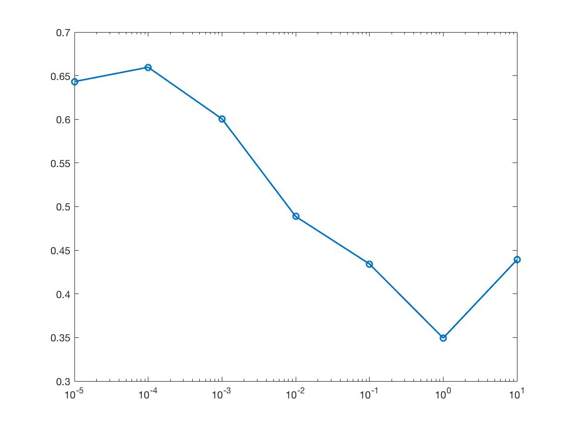
Given the results, a lambda value of 0.0001 was used throughout the project.
Extra Credit
Spatial Pyramid Features
Bag of SIFT features performed well, but like normal SIFT features, they lost all spatial information any image had. Some of this information can be preserved by splitting an image into a 4x4 grid and computing the histogram of SIFT features for each cell in the grid. This could be taken even further by splitting each image into a 16 x 16 grid and repeating the process. The smaller the grid though, the sparser the histograms will be thus limiting its effectiveness.
While keeping track of some of the spatial information is great, these features can be even more complete by storing every layer of spatial information into a single feature. This obviously has the disadvantage of using up more memory and being slow to run, but can offer significant increases in accuracies. The code for creating these spatial pyramid histograms is shown here:
    height_fourth = size(img, 1) / 4;
    width_fourth = size(img, 2) / 4;

    height_sixteen = size(img, 1) / 16;
    width_sixteen = size(img, 2) / 16;

    % compute histogram
    histogram_main = zeros(1, vocab_size);
    histogram_4 = zeros(4, 4, vocab_size);
    histogram_16 = zeros(16, 16, vocab_size);

    for j=1:size(indicies,2)
        location = locations(:, j);

        x4 = ceil(location(2) / height_fourth);
        y4 = ceil(location(1) / width_fourth);

        x16 = ceil(location(2) / height_sixteen);
        y16 = ceil(location(1) / width_sixteen);

        histogram_main(indicies(j)) = histogram_main(indicies(j)) + 1;
        histogram_4(x4, y4, indicies(j)) = histogram_4(x4, y4, indicies(j)) + 1;
        histogram_16(x16, y16, indicies(j)) = histogram_16(x16, y16, indicies(j)) + 1;
    end

    histogram = [histogram_main histogram_4(:)' histogram_16(:)'];
A 2 layer spatial pyramid can achieve an accuracy of 72.5%.
A 3 layer spatial pyramid can achieve an accuracy of 72.9%.
Overall, using a spatial pyramid for features improved accuracies almost 6 percent, however it should be noted that adding layers beyond the first extra layer didn't increase accuracies a meaningful amount, and took significantly longer to compute.
Final Results
Submitted Results
The code that was submitted had a couple changed to factor in running time. The bag of SIFT step size was increased to 7 and all extra credit was removed. Here are the resulting accuracies:
| Feature | Classification | Accuracy |
|---|---|---|
| Tiny Images | Nearest Neighbor | 19.2% |
| Bag of SIFT | Nearest Neighbor | 50.5% |
| Bag of SIFT | SVM | 66.5% |
Spatial Pyramid Bag of SIFT with SVM Classifier
Scene classification results visualization
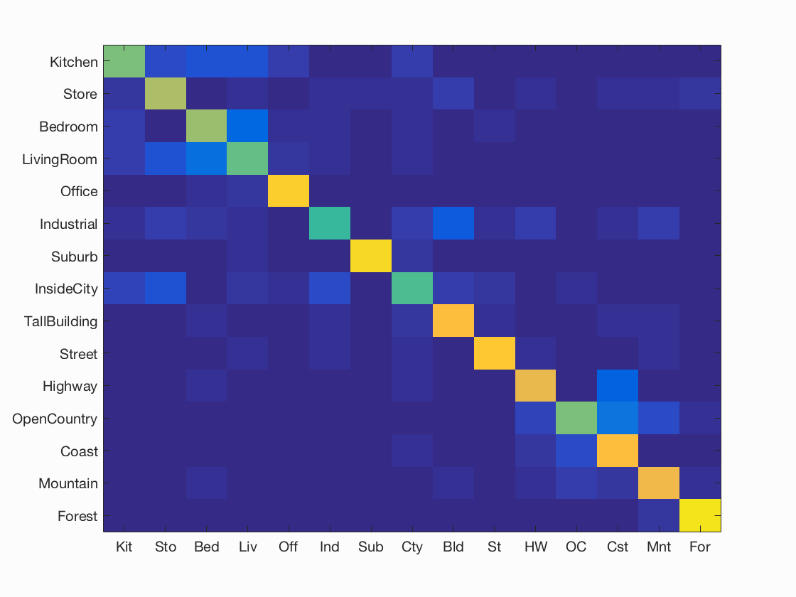
Accuracy (mean of diagonal of confusion matrix) is 0.735
| Category name | Accuracy | Sample training images | Sample true positives | False positives with true label | False negatives with wrong predicted label | ||||
|---|---|---|---|---|---|---|---|---|---|
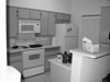
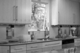
| Kitchen | 0.600 | 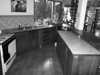 |
 |
 |
 |
 InsideCity |
 Store |
 Office |
 Store |
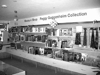
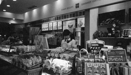
| Store | 0.680 | 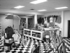 |
 |
 |
 |
Kitchen |
 LivingRoom |
 Kitchen |
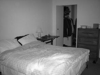
| Bedroom | 0.650 | 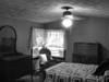 |
 |
 |
 |
 Kitchen |
 LivingRoom |
 Industrial |
 Kitchen |
| LivingRoom | 0.570 | 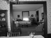 |
 |
 |
 |
 InsideCity |
 Industrial |
 Bedroom |
 Industrial |
| Office | 0.890 |  |
 |
 |
 |
 Store |
 Kitchen |
 LivingRoom |
 LivingRoom |
| Industrial | 0.510 | 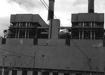 |
 |
 |
 Office |
 Bedroom |
 Kitchen |
 Forest |
|
| Suburb | 0.920 | 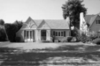 |
 |
 |
 |
 Highway |
 Store |
 LivingRoom |
 InsideCity |
| InsideCity | 0.540 |  |
 |
 |
 |
 Coast |
 LivingRoom |
 Street |
 Forest |
| TallBuilding | 0.830 |  |
 |
 |
 |
 Mountain |
 InsideCity |
 Industrial |
 Industrial |
| Street | 0.860 |  |
 |
 |
 |
 Office |
InsideCity |
 InsideCity |
 Highway |
| Highway | 0.790 |  |
 |
 |
 |
 Industrial |
 OpenCountry |
 Coast |
 Industrial |
| OpenCountry | 0.600 |  |
 |
 |
 |
 InsideCity |
 Coast |
 Coast |
 Coast |
| Coast | 0.840 |  |
 |
 |
 |
 OpenCountry |
 Highway |
 OpenCountry |
 Highway |
| Mountain | 0.810 |  |
 |
 |
 |
 Forest |
 OpenCountry |
 Coast |
 Street |
| Forest | 0.940 |  |
 |
 |
 |
 Store |
 Store |
 Mountain |
| Category name | Accuracy | Sample training images | Sample true positives | False positives with true label | False negatives with wrong predicted label | ||||