Project 4 / Scene Recognition with Bag of Words
The goal of this project was to explore three different pipelines for scene recognition in images.
Tiny Image Representation with Nearest Neighbor Classifier
The first pipeline tested was using the "tiny image" feature to describe images, followed by a nearest neighbor (1NN) classifier to match the test images with the training images. Implementing the tiny image representation was simply a matter of resizing each image to 16x16 pixels and vectorizing them so they can be used as featuers. The vector representation of the tiny image was also normalized to zero mean and unit length to improve accuracy.
The 1NN classifier was also fairly straightforward. The pairwise distances between training and test image features were computed and sorted. The top results would be the nearest neighbor in the set of training images to each test image. The category corresponding to the selected training image was then assigned to test image.
This pipeline achieved 23.8% accuracy. There were no parameters to tune in this pipeline.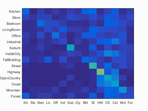
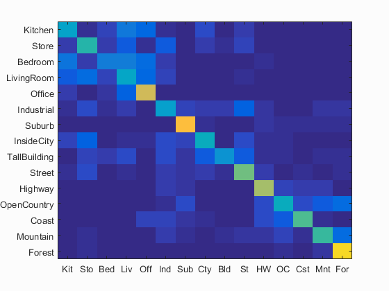
Bag of SIFT Representation with Nearest Neighbor Classifier
The second pipeline tested was using the bag of SIFT features to represent images, followed by the same 1NN classifier from the first pipeline. In order for the bag of SIFT representation to work, a vocabulary of visual words had to be created. This was done by sampling tens of thousands (30,000 in my case) of SIFT features from the set of training images and then grouping them with kmeans clusutering. Larger samples were experimented with, but while they showed improved accuracy, it was insignificant and modestly increased the runtime.
Once the vocabulary was created, bags of SIFT features were constructed by sampling SIFT features from test images at a much denser rate than when building the vocabulary. For the sake of runtime, however, the bag was restricted up to a maximum number of features m; more features resulted in improved accuracy, however. The pairwise distances between the bag of SIFT features and vocabulary were computed and sorted. A histogram was then made from the number of instances in which each vocabulary visual word was selected as the nearest neighbor for every feature in the bag of SIFT features. Finally, the histogram was normalized and stored to represent each test image when it undergoes classification.
This pipeline achieved 51.4% accuracy with m = 20 inbuild_vocabulary.m, m = 1500 in get_bags_of_sifts.m, and vocab_size = 200 in proj4.m.
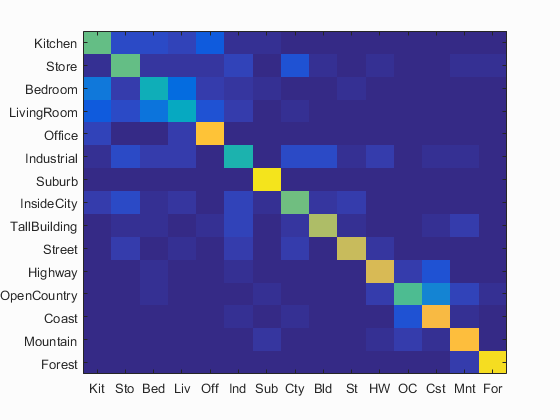
Bag of SIFT Representation with Linear Support Vector Machine Classifier
The third pipeline tested was using the bag of SIFT features from the second pipeline, followed by linear SVM classifiers. The task was to train 1-vs-all linear SVMs in to work in the bag of SIFT feature space. Each linear SVM corresponds to one of the 15 scene categories. The binary labels for each training image in every category (whether the test image matches the corresponding scene or not) were initialized to -1, and each training labels that matched the current categroy was set to 1. VLFeat's vl_svmtrain function was then used to train the linear SVM given training image features, labels, and a regularization parameter λ (some testing showed that 0.00005 appeared to give roughly optimal results). This function returns a vector of weights for each corresponding image feature and an offset used to calculate the confidence of each image in every scene category. Finally, each image was assigned its most confident scene category label.
build_vocabulary.m, m = 1500 in get_bags_of_sifts.m, vocab_size = 200 in proj4.m, and λ = 0.00005 in svm_classify.m.
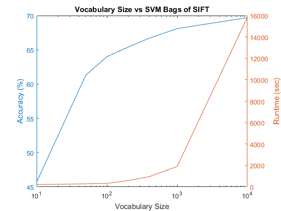
Experimenting with Vocabulary Size
It was found that increasing vocabulary size improved accuracy to an extent, but the improvement tapers rapidly while dramatically increasing runtime to complete the full pipeline, including building the vocabulary.
Final scene classification results visualization
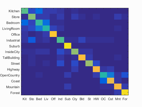
Accuracy (mean of diagonal of confusion matrix) is 69.7% with m = 20 in
build_vocabulary.m, m = 1500 in get_bags_of_sifts.m, vocab_size = 10,000 in proj4.m, and λ = 0.00005 in svm_classify.m.
| Category name | Accuracy | Sample training images | Sample true positives | False positives with true label | False negatives with wrong predicted label | ||||
|---|---|---|---|---|---|---|---|---|---|
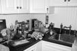
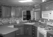
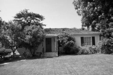
| Kitchen | 0.560 |  |
 |
 |
 |
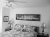
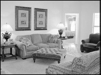
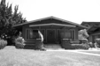
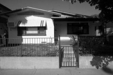
 Bedroom |
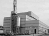
 Industrial |
 Bedroom |
 Industrial |
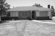
| Store | 0.610 | 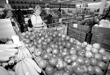 |
 |
 |
 |
 Industrial |
 Bedroom |
 InsideCity |
 Kitchen |
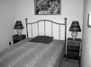
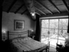
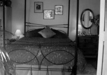
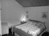
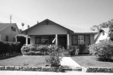
| Bedroom | 0.510 |  |
 |
 |
 |
 Office |
 Kitchen |
 LivingRoom |
 Kitchen |
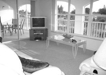
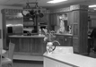
| LivingRoom | 0.480 | 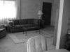 |
 |
 |
 |
 Bedroom |
 Kitchen |
 Bedroom |
 Industrial |
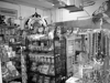
| Office | 0.860 |  |
 |
 |
 |
 Kitchen |
 Kitchen |
 Bedroom |
 LivingRoom |
| Industrial | 0.540 |  |
 |
 |
 |
 Store |
 Street |
 InsideCity |
 TallBuilding |
| Suburb | 0.950 | 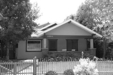 |
 |
 |
 |
 OpenCountry |
 OpenCountry |
 OpenCountry |
 Coast |
| InsideCity | 0.640 |  |
 |
 |
 |
 Street |
 Kitchen |
 Street |
 Bedroom |
| TallBuilding | 0.830 |  |
 |
 |
 |
 Industrial |
 Street |
 Coast |
 Industrial |
| Street | 0.650 |  |
 |
 |
 |
 InsideCity |
 Bedroom |
 Industrial |
 Mountain |
| Highway | 0.820 |  |
 |
 |
 |
 LivingRoom |
 Street |
 Coast |
 OpenCountry |
| OpenCountry | 0.470 |  |
 |
 |
 |
 Coast |
 Mountain |
 Mountain |
 Coast |
| Coast | 0.790 |  |
 |
 |
 |
 OpenCountry |
 OpenCountry |
 OpenCountry |
 Mountain |
| Mountain | 0.820 |  |
 |
 |
 |
 Forest |
 TallBuilding |
 Suburb |
 Street |
| Forest | 0.930 |  |
 |
 |
 |
 Mountain |
 OpenCountry |
 Mountain |
 Mountain |
| Category name | Accuracy | Sample training images | Sample true positives | False positives with true label | False negatives with wrong predicted label | ||||