Project 4 / Scene Recognition with Bag of Words

Image representation / Features

The first step in image recognition is to construct an image representation that will be used to train the classification algorithm. A simple image representation is tiny images, which is a small-scale version of the original image. The tiny images representation used in this project is a 16 x 16 feature normalized to a zero to one range.

%Tiny images
I = imresize(I,[16,16]);
I = reshape(I,1,256);
I = (I - min(I)) / (max(I) - min(I));

To obtain a more complex representation of images, we can use the bag of words model with SIFT features. The process involves computing SIFT features throughout a given image and using K-means to cluster the features into a "vocabulary". Next, a bag of words representation is used which involves building a histogram of the occurrence of each visual word. The resulting feature will have the same dimension as the number of visual words in the vocabulary.

%Bag of SIFT
[~, SIFT_features] = vl_dsift(I,'step',10,'fast');
image_feats(:,(i-1)*numSample+1:i*numSample) = SIFT_features(:,randi(numFeatures,numSample,1));
[vocab, ~] = vl_kmeans(image_feats, vocab_size);
model = KDTreeSearcher(vocab);
[id,~] = knnsearch(model,single(SIFT_features'),'K',1);
for j=1:length(id)
	image_feats(i,id(j)) = image_feats(i,id(j)) + 1;
end

Classifier

The next step is to use a machine learning classifier to predict the class label for each test image given the training image features, training image labels and the test image features. One simple method is to use nearest neighbors, where the predicted label is computed directly from the training data point which is closest to the query data in feature space.

%Nearest neighbor
model = KDTreeSearcher(train_image_feats);
[id,~] = knnsearch(model,test_image_feats,'K',k);
predicted_categories = train_labels(id);

Another possible classifier is the Support Vector Machine (SVM) classifier. This project uses Linear SVM, which calculates a separating hyperplane in feature space for a given positive class versus a negative class. To enable multi-class classification, the one-vs-all scheme is used, where multiple SVM classifiers are trained with positive training examples from each class and negative training examples from the remaining classes. At test time, the predicted class is determined from the classifier with the highest score/confidence.

%SVM
for c=1:num_categories
    labels = strcmp(categories(c), train_labels) * 2 - 1;
    [W(:,c),B(1,c)] = vl_svmtrain(train_image_feats', labels, lambda);
end
score = test_image_feats * W + repmat(B,N,1);
[~,index] = max(score, [], 2);
predicted_categories = categories(index);

The experimental results are shown in the table below. Note that the measured accuracy will vary depending on system parameters such as number of sampled SIFT features, sampling density and vocabulary size. The results reported below are for #samples=1000, sampling step=10, vocabulary size=1000, #neighbors = 1, lambda (for SVM) = 0.001.

Method	Accuracy
Tiny images + Nearest Neighbor	0.220
Bag of SIFT + Nearest Neighbor	0.457
Bag of SIFT + Support Vector Machine	0.637

Soft assignment (Extra Credit)

The method of histogram binning for computing the bag of words representation tends to lead to over-discretization. This problem can be handled using soft assignment, where the query feature casts not a single, but multiple weighted votes to each of its nearest neighbors in feature space. The method used in this project is to weight each vote according to the exponential of the distance in feature space, also known as kernel codebook encoding (shown below).

%Soft assignment
[~, SIFT_features] = vl_dsift(I,'step',10,'fast');
[id,dist] = knnsearch(model,single(SIFT_features'),'K',K);
for j=1:length(id)
	for k=1:K
		vote = exp(-beta*dist(j,k));
		image_feats(i,id(j,k)) = image_feats(i,id(j,k)) + vote;
	end
end


The distribution of weights depend on the beta parameter, which controls the smoothness across each vote. The recognition accuracy is reported below for
bag of SIFT (vocabulary size = 50) + soft assignment + SVM with different values of beta. The results indicate that in general, the accuracy increases as the value of
beta decreases, which means that each assignment casts votes with more similar weights.


Beta
Accuracy
1e-1
0.067
1e-2
0.343
1e-3
0.385
1e-4
0.383


Fisher Encoding (Extra Credit)
One possible improvement that can be made to the bag of words model is to use a more sophisticated encoding scheme such as Fisher encoding. The distribution of training feature vectors
is first modeled as a Gaussian Mixture Model with K clusters. Next, the training and test features are encoded based on the computed priors, means, and covariances for each cluster.
Finally, a linear SVM classifier is trained based on the Fisher vectors and used to predict class labels.

%Fisher Encoding
[means, covariances, priors] = vl_gmm(image_feats, numClusters);
for i=1:N
    enc = vl_fisher(image_feats(:,(i-1)*numSample+1:i*numSample), means, covariances, priors,'improved');
    train_image_feats(i,:) = enc';
end


The recognition accuracy is reported below as a function of the number of clusters used in the GMM estimation.The results show that in general, the accuracy increases with the number of clusters.


Number of clusters (K)
Accuracy
10
0.617
20
0.647
50
0.647
100
0.669
500
0.701


Improved Nearest Neighbor(Extra Credit)
According to Boiman, Schechtman, and Irani (CVPR 2008), the method of nearest neighbors applied directly on image features can be used for classification
to avoid the problem of over-discretization. This is because conventional methods using bag of words only capture the histogram of image features for a fixed number
of visual words while the original features are lost. On the other hand, the proposed method stores the features for all the training data and finds the nearest neighbor
match for test image features. For each test image, the predicted class is determined as the class which minimizes the total distance in feature space for nearest neighbor
matches within that class.

%Improved nearest neighbor
for c=1:num_categories
	feats_c = train_image_feats(strcmp(categories(c), train_labels),:);
	model = KDTreeSearcher(feats_c);
	[~,dist] = knnsearch(model,test_image_feats,'K',1);
	sumDist = sum(reshape(dist,numSample,[]))';
	ind = find(sumDist < minDist);
	minDist(ind) = sumDist(ind);
	predicted_categories(ind) = c;
end


The recognition accuracy is reported below as a function of the number of sampled features per image. The results show that the accuracy increases with the number of sampled features per images.
It is expected that with a large enough number of sampled features, this method can be competitive or better than linear SVM.


#Sampled features per image
Accuracy
10
0.257
50
0.450
100
0.519


Cross Validation (Extra Credit)
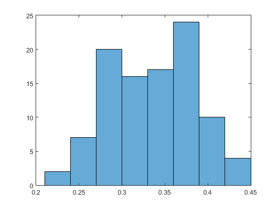
To overcome the problem of outliers in the data, a more reasonable way to measure recognition accuracy is to employ cross validation. Instead of measuring
the accuracy on the entire training and testing data set, a randomly sampled subset of the training data is selected along with a randomly sampled subset of the test data
to measure the recognition accuracy. This is repeated several times to obtain a distribution over the recognition performance. The results for bag of SIFT + SVM
with a vocabulary size=50, sample size=100 #iterations=100 is shown in the figure below (x-axis is accuracy, y-axis is frequency). The mean accuracy is 0.33 while the standard deviation is 0.05.




Effect of vocabulary size (Extra Credit)
 This section aims to investigate the effect of vocabulary size on the recognition accuracy of the bag of SIFT image representation. 
The vocabulary size is increased from 10, 20, 50, 100, 200, 400, to 1000 and the accuracy and computation time are recorded in the table below.
The experiments were carried out using the bag of SIFT image representation with SVM classifier.
The results show that in general, as the vocabulary size increases, the accuracy increases but this comes at the cost of higher computation time.


Vocabulary Size
Accuracy
Computation Time (s)
10
0.219
51.85
20
0.375
62.34
50
0.443
84.57
100
0.541
125.87
200
0.552
187.05
400
0.585
353.57
1000
0.637
808.14


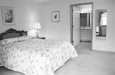
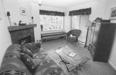
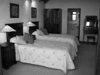
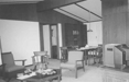
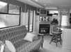
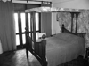
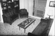
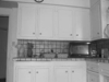
Scene classification results visualization

The best results were obtained using Fisher encoding + linear SVM with 1000 samples features per image and 500 clusters.





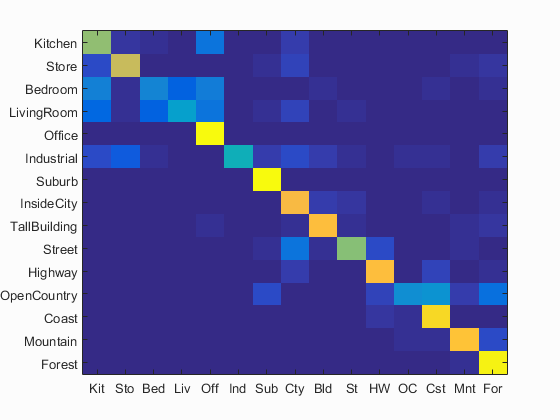
Accuracy (mean of diagonal of confusion matrix) is 0.701




Category name
Accuracy
Sample training images
Sample true positives
False positives with true label
False negatives with wrong predicted label


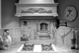
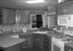
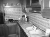
Kitchen
0.640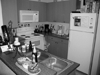





Bedroom

Bedroom

InsideCity

Office


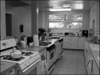
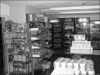
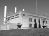
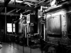
Store
0.720





Kitchen

Industrial

Suburb

Street


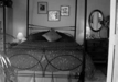
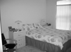
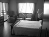
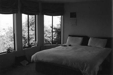
Bedroom
0.250





Industrial

LivingRoom

LivingRoom

LivingRoom


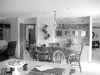
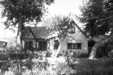
LivingRoom
0.350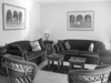





Bedroom

Bedroom

Kitchen

Bedroom


Office
0.990





Kitchen

TallBuilding

Kitchen



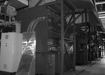
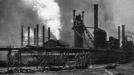
Industrial
0.430





Kitchen

Bedroom

Suburb

Store


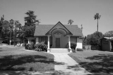
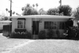
Suburb
1.000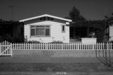





Industrial

Mountain




InsideCity
0.820





Street

Store

TallBuilding

Suburb


TallBuilding
0.840





Bedroom

OpenCountry

Office

InsideCity


Street
0.620





InsideCity

InsideCity

Kitchen

Highway


Highway
0.830





Street

Street

Coast

Coast


OpenCountry
0.290





Coast

Coast

Coast

Coast


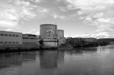
Coast
0.920





Bedroom

Highway

OpenCountry

Highway


Mountain
0.850





TallBuilding

TallBuilding

Forest

OpenCountry


Forest
0.970





InsideCity

Store

Street

Mountain


Category name
Accuracy
Sample training images
Sample true positives
False positives with true label
False negatives with wrong predicted label