Project 4 / Scene Recognition with Bag of Words
Quick Summary
Basic Implementation
- Tiny image features.
- 1-NN.
- Get Vocabulary/li>
- Bags of features
- 1-vs-all SVM
Extra Implementation
- TF-IDF
- Gist
- Validation for hyper-parameter tuning
- Cross-Validation for performance evaluation
- spatial pyramid
- test of different vocabulary sizes
For tiny patch, I just use imresize function to compress the original images to 16x16 tiny image. For nearest neighbor, I use the basic one nearest neighbor approach to assign each feature to its nearest center. The accuracy for 1-NN approach plus tiny patch is quite low. If using SVM plus tiny patch, slightly better, about 20%
Then I used bag of features approach. After trying different parameters for vl_dsift, I found that the bin_size = 6, step = 15 is OK. However if I use vl_sift function, the accuracy is very low.
Condition: Bags of features, 1NN:
BinSize = 3,ACC = 0.424
BinSize = 4 ACC = 0.440
BinSize = 5 ACC = 0.443
BinSize = 6 ACC = 0.443
Then I implemented spatial pyramid and get the accuracy using 1-vs-all SVM. Basically, for each image, after extracting its all sift features, I will call a function call get_histo to compute the histogram of the features assigned to each visual word. This function will accept a list of coordinates of sift features, and a parameter K, which is maximum spatial pyramid layer number. This function would first compute the histogram using all those coordinates, and then will recursively call itself for 4 times. Each time, it will pass a subset of the coordinates and a K-1 layer parameter. So if the number visual words is 200, a 1 layer pyramid would have 200 features, two layers pyramid has 1000=200+200*4 features, three layers pyramid has 4200= 200 + 200*4 + 200*4*4. Shown below, adding spatial information approach do give a huge improvement. However, it is not always the case that the more layers, the better accuracy. Here the 3 layers pyramid is the optimal one. So for later experiments, I used 3 layers.
Condition: bags_of_features, 200_visual_words, 1_vs_all_SVM.
1-layer, 200 features: ACC 0.497
2-layers, 1000 features: ACC 0.600
3-layers, 4200 features: ACC 0.644
4-layers, 17000 features: ACC 0.623
Then I implemented validation and cross-validation. For explicity, the validation here is used for tuning the hyper-parameters, whereas Cross-validation is used for report the stability of a certain hyper-parameter.
In validation procedure, I first randomly shuffle the original training dataset and then split it into two subsets, training and validation. The ratio of the number of samples in training set to that in validation set is 2:1. Then I create a hyper-parameter matrix in which rows represesnt a combination of hypameters which would be used in a 1-vs-all SVM cluster. More concretely, each 1-vs-all SVM has a regularization parameter. To predict all 15 categories, we need 15 SVMs, which form a cluster. In my hyper-parameter matrix, each row contains 15 parameter which should be used for the 15 SVMs cluster. After iterating through each row, I can find the best parameter combination.
Here is the current matrix, and the best results. It can be seen that the accuracies at the upper-left corner is not good enough.
Hyper-parameter matrix:
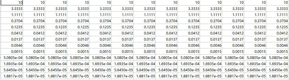
Condition: 3-layers, 4200 features:
Untuned hyper-parameter: ACC 0.644
Turned hyper-parameter: ACC 0.686
Though current I have do not enough time to test, it can be imagined that by modifying the default hyper-parameter matrix, the SVMs for the first 3 class would have different performances, and finally the overall performance at the upper-left corner would be better.
After getting the best hyper-parameter combination, it is the time for cross-validation
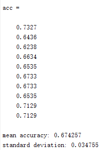
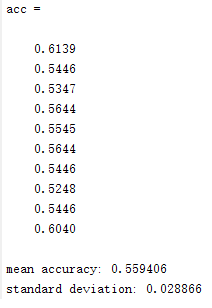
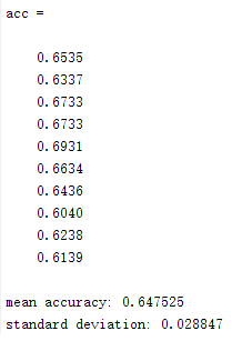
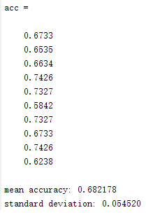
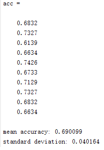
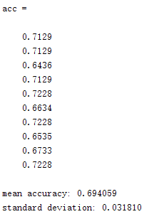
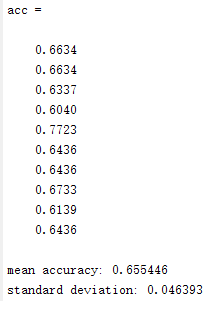
In my implementation, cross-validation has 10 repeats. In each repeats, it first randomly shuffles the training data, select 100 samples as validation set and leave others as training set. It will use the best hyper-parameter combination for the 15 SVMs.After getting the 10 accuracies, it would calculate their mean and standard deviation.
Accuracies in each iteration and their overall mean and STD.
sample images correspond to different sizes of vocabularies, 10, 20, 50, 100 and 200. Detailed vocabularies tests are shown be;pw.
Size 10: ACC 0.591
Size 20: ACC 0.624
Size 50: ACC 0.667
Size 100: ACC 0.656
Size 200: ACC 0.686
Size 400: ACC 0.692
Size 1000: ACC 0.668
I also implemented TF-IDF and Gist feature. However, the two did not give a significant improvement. So, just a quick description here.
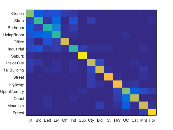
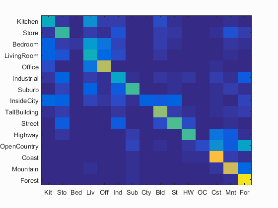
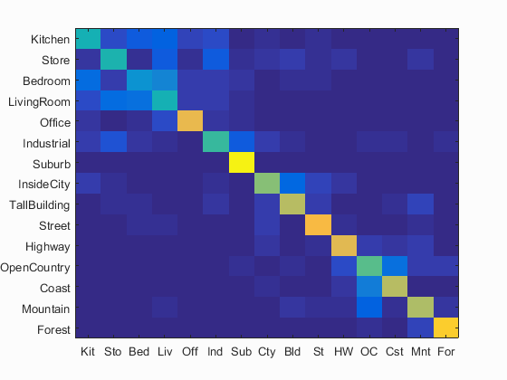
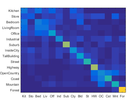
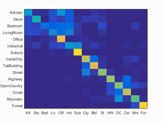
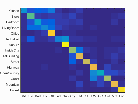
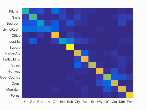
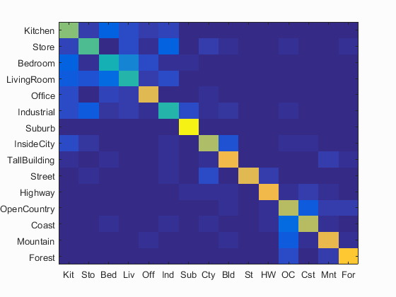
Some awkward result:
Left: No TF-IDF
Right: with TF-IDF
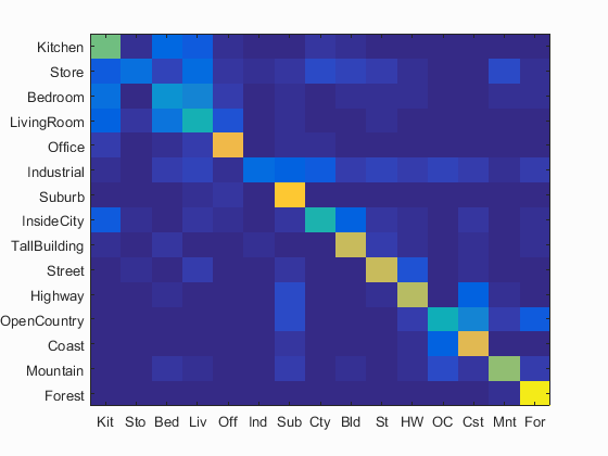
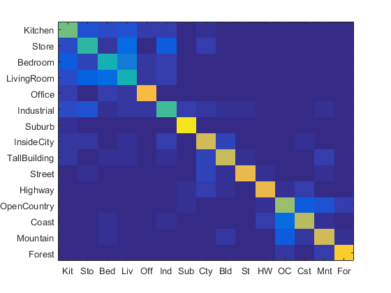
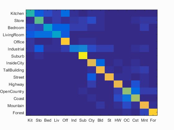
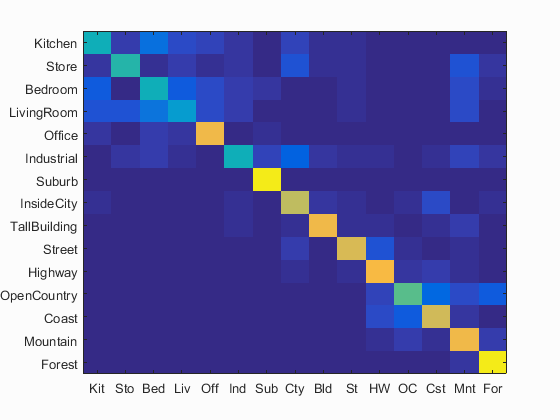
Left: Sift_Only
Right: Sift + Gist