Project 4: Scene Recognition with Bag of Words
First we will go over the overview of what I implemented and how (please feel free to reference full code in matlab files). Then I will show and discuss my results for different combinations of features and classifiers. We will also talk a bit more about my choice of parameters and how/why I chose the parameters I did.
Part 1: Tiny Image Feature
For the tiny image representation implementation I simply resized my images to be of a small fixed resolution. For this project I used 16x16. I also made sure that the image had zero mean and unit length. The core of the code resizes the image and then normalizes it. This code is applied to each image and is shown below:
resized_image = imresize(image, [16 16]);
results = im2double(reshape(resized_image, [1,256]));
final_feats(image_num,:) = results ./ norm(results);
In this section of the project I experimented with other sized patches like 8x8 and 12x12 but I found that 16x16 worked best while still being quite fast.
Part 2: Nearest Neighbor Classifier
For this portion I implemented a very simple nearest neighbor classifier. This classifier simply finds the closest neighbor for a feature and returns that classification. The nice thing about this is that it requires no training and is very fast. From an implementation standpoint the crux of the implementation was calculating all the distances between features ahead of time and then simply taking the min distance for each feature in the test set. The code to precompute these distances is shown below:
distances = vl_alldist2(train_image_feats', test_image_feats');
In terms of modifying parameters, here my main consideration was using multiple nearest neighbors to vote on a classification. For instance we could take the 3 closest neighbors and have them vote on a classification, defaulting to the nearest neighbor if all 3 are different classifications. For the purposes of this simplistic method, I kept it as only the neraest neighbor as there was a very minimal change in accuracy by considering more neighbors.
Part 3: Bags of Quantized SIFTs (and building vocabulary)
First, I built the vocabulary. There were a lot of parameters to account for here. Through much testing I chose to sample 50,000 features and build a vocabulary of size 200. I wanted the size to be sufficient but still not take too long to run. A size of 200 allowed for 200 cluster centers in k means clustering, which I felt from testing was a good amount based on my sample size of 50,000. I found that with numbers closer to 10,000 with my sample size my accuracy decreased because my centers didn't have enough information. I found that too many features required a larger vocabulary and ran very very slowly. The code below shows how I determined how many features I wanted to sample per image, and then shows how I obtained the SIFT_features.
total_features = 50000;
feat_per_img = ceil(total_features/size(image_paths,1));
% ...
% the following code is in a loop through the images
[locations, SIFT_features] = vl_dsift(image_single, 'step', 10, 'fast');
Here we see another key paramtere of step size!! The lower the step size the more often features will be extracted from an image. This means that a small step size makes the code extremely slow. I found that be having a step size of 10 my code did not take too too long to build a vocabulary and still sampled enough features to where my vocabulary produced good results! I also found that modifying step size was very important to determining different results. I think that having a step size too small sampled an image too frequently, and generally for me a higher step size did a better job of generalizing and building a vocabulary that did not overfit to the training set!
Once I built the vocabulary I could create the bag of quantized SIFTs feature! For each image I sampled many SIFT descriptors. I then used a distance measure to determine which centroid in my vocabulary the feature was closest to. Through this approach I created a histrogram for each image of the size of my vocabulary. Thus for my 200 sized vocabulary I had a histrogram of size 200 counting how many times each of the SIFT features fell into a bin (determined by distance from the centroid). Finally, I normalized the histogram so that image size did not play a factor! I found that normalizing the histrogram improved my results by around 15%! Below is the code extracting SIFT features and computing distances:
[locations, SIFT_features] = vl_dsift(image_single, 'step', 4, 'fast');
D = vl_alldist2(vocab', single(SIFT_features));
Once again we notice this step parameter! I tested various step sizes ranging from 2 to 20. I found that a step size like 2 was far too slow for our purposes and that a step size of 20 did not extract nearly enough features for us to construct a good histrogram representation. I found that step sizes of 4-8 worked fairly well, with 4 being the clear winner in performance. This is logical as it allows us to sample the image more densly.
Part 4: 1vsALL linear SVM classifiers
Here I created a 1vsALL classifier using SVM. The idae here is to partition a feature space using a learned hyperplane. Once we have this trained division we then classify test cases. This helps us get through the issue with nearest neighbors where many of the visual words in our bag of SIFT representation may not be informative. For this project I created 15 classifiers, one for each of our classifications, where I learn a classifier for each classification versus its inverse. We take confidences that we determine from our model to determine the best classification based on which model has the highest confidence of classification. The main free parameter here is lambda, which controls how strongly regularized the model is. I found that lower lambdas made the code run slower but produce far better results, often improving by as much as 8%. My code ran quite fast with a lambda of 0.001 and acheived around 61% accuracy. By using a lambda of 0.0001, my code took nearly twice as long to run but had an accuracy of 68% of average! Below is the crux of my code where I am evaluating a single classifer's confidence for a single image:
bin_labels = -1 * ones(size(train_labels));
indices = strcmp(train_labels, categories(cat_num));
bin_labels(indices) = 1;
[W B] = vl_svmtrain(train_image_feats', bin_labels, 0.0001);
results(cat_num) = dot(W', test_image_feats(img_num,:)') + B;
The lower a lambda value (closer to 0) the more misclassifications are allowed by our model. By having a smaller lambda we can allow our model to generalize well. With a lambda value too small, however, we allow too many misclassifications are don't fit our information well enough. I was able to achieve around 68% accuracy, as discussed further below!
Examining Results for Various Feature/Classifer Pairs
Below is the accuracy (defined as the accuracy number reported by the starter code, or the average of the diagonal of the confusion matrix) I achieved for the three recognition pipelines specified in the instructions:
- tiny images + nearest neighbor: 20.0%
- bag of SIFT + nearest neighbor: 51.5%
- bag of SIFT + 1 vs all linear SVM: 68.5%
First lets discuss the parameters used to achieve these results before looking at the confusion matrix and tables produced for my best pipeline. For the tiny images with nearest neighbor I used 16x16 tiny images normalized and single nearest neighbor as a classifier. For the building of vocabulary for both the 2nd and 3rd pipelines I used 50,000 samples with a vocabulary size of 200, and using a step size of 10 and the 'fast' parameter. For the bag of SIFT + nearest neighbor, I used a step size of 8 again with the 'fast' parameter, with the same nearest neighbor algorithm mentioned above. I used this step size for speed not because it had the best accuracy (I had better accuracy with lower step sizes). I also normalized the histograms for bag of SIFT. For the final pipeline, I used a step size of 4 for bag of SIFT with the 'fast' parameter, agian normalizing the histograms. For the 1vALL SVMs I used lambda value of 0.0001. What is very important to note is that this is DIFFERENT than what is turned in, because this pipeline took logner to run. I used a step size of 8 and a lambda value of 0.001 to increase the speed in the assignment turned in! Using a step size of 8 and this higher lambda value, my accuracy for bag of SIFT + 1 vs all linear SVM was 58.7%. This varied each run but only by a very small amount.
Below are the confusion matricies for the first two pipelines, with the final pipeline shown in more detail afterwards.
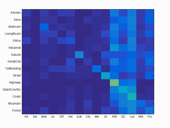
tiny images + nn |
bag of SIFT + nn |
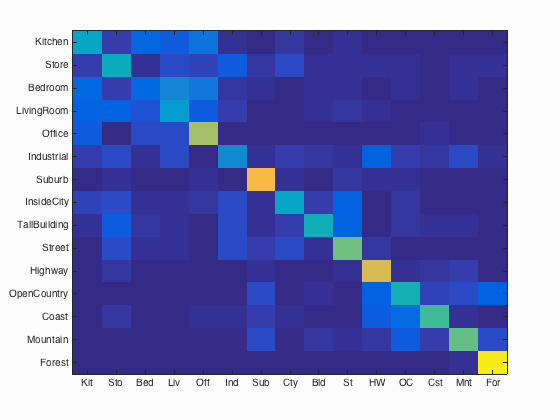
My best performing pipeline was using the final configuration mentioned, and the full confusion matrix and the table of classifier results produced by the starter code are shown below!
Scene classification results visualization: bag of SIFT + 1 vs all linear SVM

Accuracy (mean of diagonal of confusion matrix) is 0.685
| Category name | Accuracy | Sample training images | Sample true positives | False positives with true label | False negatives with wrong predicted label | ||||
|---|---|---|---|---|---|---|---|---|---|
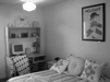
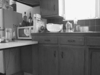
| Kitchen | 0.670 |  |
 |
 |
 |
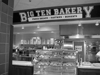
 Store |
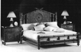
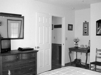
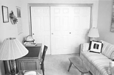
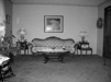
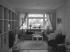
 Bedroom |
 Bedroom |
 Store |
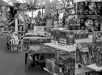
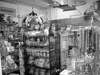
| Store | 0.500 |  |
 |
 |
 |
 Bedroom |
 InsideCity |
 Office |
 InsideCity |
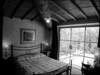
| Bedroom | 0.430 |  |
 |
 |
 |
 LivingRoom |
 LivingRoom |
 LivingRoom |
 Store |
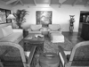
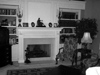
| LivingRoom | 0.410 |  |
 |
 |
 |
 Bedroom |
 Street |
 Bedroom |
| Office | 0.890 |  |
 |
 |
 |
Store |
 Kitchen |
 Kitchen |
 Kitchen |
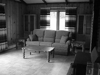
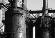
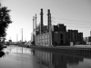
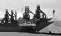
| Industrial | 0.450 |  |
 |
 |
 |
 TallBuilding |
 Store |
 Store |
 Coast |
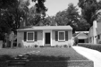
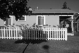
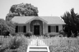
| Suburb | 0.960 |  |
 |
 |
 |
 Industrial |
 LivingRoom |
 Street |
 OpenCountry |
| InsideCity | 0.610 |  |
 |
 |
 |
 Highway |
 LivingRoom |
 Store |
 Suburb |
| TallBuilding | 0.820 |  |
 |
 |
 |
 Industrial |
 Industrial |
 Bedroom |
 Kitchen |
| Street | 0.720 |  |
 |
 |
 |
 TallBuilding |
 Industrial |
 InsideCity |
 Industrial |
| Highway | 0.830 |  |
 |
 |
 |
 OpenCountry |
 OpenCountry |
 Mountain |
 OpenCountry |
| OpenCountry | 0.460 |  |
 |
 |
 |
 Mountain |
 Street |
 Coast |
 Forest |
| Coast | 0.760 |  |
 |
 |
 |
 OpenCountry |
 OpenCountry |
 Mountain |
 OpenCountry |
| Mountain | 0.820 |  |
 |
 |
 |
 OpenCountry |
 OpenCountry |
 Suburb |
OpenCountry |
| Forest | 0.940 |  |
 |
 |
 |
OpenCountry |
 Highway |
 Mountain |
 Mountain |
| Category name | Accuracy | Sample training images | Sample true positives | False positives with true label | False negatives with wrong predicted label | ||||