Project 4 / Scene Recognition with Bag of Words
For this project, the main goal was to label images into the right category based on the scene that it was a part of by describing the image and utilizing a machine learning classification technique to train on a group of test images, and then test on a group of testing images. Techniques started off with simple methods (tiny images and nearest neighbor classification) to more complex methods (bags of features and linear classifiers based on support vector machines).
Tiny Image Representation and Nearest Neighbor Classifier
The first method of image feature representation that was attempted was the tiny image representation. The tiny image feature is very simple, as it simply resizes each image to a fixed small resolution, and uses that as the descriptor for the image. In this case, a size of 16x16 was chosen. Images not of this resolution were scaled so that they fit within the 16x16 pixel constraint. This feature description technique was then paired with the nearest neighbor classifier to determine what label to classify a test image with. 1-nearest neighbor simply finds the nearest training example that matches up to the current text case, and assigns that test case the same label of the nearest training example. The distance calculation method used was L2 distance. Another technique that could have been implemented would be K-nearest neighbor, which can help alleviate training noise by voting based on the k nearest neighbors rather than one, however, this was not implemented as part of this project. The results of these two techniques paired together resulted in an accuracy of roughly 22.5%, which is better than the random chance categorization of ~7%.
Bag of Features and Nearest Neighbor Classifier
The second method of feature representation chosen was the Bag of SIFT features representation. In order to utilize this technique, a vocabulary of visual words had to be created first. The vocabulary was formed by sampling local features from the training set (using SIFT features) and then clustering them with kmeans and a certain number of clusters. In this case, a varying amount of features were used (generally between 200 to 1000) per image, and a k-means cluster size of generally around 200 (with different values for experimental purposes). Higher amounts of features were also tested upon (such as 500 and 1000), but the amount did not seem to affect the end results by much. This is likely because with 200 features of each of the 1500 images in the training set likely resulted in enough features such that more would only cause redundancy. The final clusters of kmeans results in the size of our vocabulary and features. Any new SIFT features determined can then be classified into the nearest cluster that it belongs to, which we can then use with a distance function to determine what the test case image should be labeled with.
After the vocabulary was determined, we run our training set through the bag of words descriptor, and use all features associated with the images. For each image in the training set, we determine how many of the SIFT features fall into each cluster determined by the k-means process earlier from our vocabulary. The test images are then run through the same bag of words descriptor and the same vocabulary used for training, and we determine how many of the SIFT features for each of the test images fall into each cluster determined by k-means. Thus, the images are being described by how many of their features fall into the vocabulary clusters determined earlier. The resulting vector is then normalized to account for differences in image sizes (as larger images would tend to have more SIFT features, meaning that the resulting descriptor would have more values overall classifed into the vocabulary clusters). Finally, this is paired with nearest neighbor (with L2 distance calculation) between all images in training and testing sets to determine what image in the training set the test case is most similar to. The test case is then given the same label as the training image. This resulted in an accuracy of around 55%. The code below for determining the bag of features descriptors is shown partly below, where it obtains SIFT features from the images and places them into the nearest vocabulary cluster.
% obtain SIFT features
[locations, SIFT_features] = vl_dsift(single(img), 'Fast', 'Step', 10);
locations = locations';
SIFT_features = SIFT_features';

% calculate distance from features to vocab
distance = vl_alldist2(vocab', double(SIFT_features'));
[sorted, indexes] = sort(distance);
feature_vector = double(zeros(1, vocab_size));
for j = 1:size(sorted, 2)
   min = sorted(1, j);
   min_index = indexes(1, j);
   feature_vector(1, min_index) = feature_vector(1, min_index) + 1;
end
Bag of Features Linear Support Vector Machine
This technique changes the classifier technique only, so the bag of features method is still used from previous. However now, a 1-vs-all linear support vector machine was trained on the bag of SIFT features. Since linear classifiers can only be used between two identifiers, a linear SVM for each individual scene category had to be used, which compared that specific scene to all examples that were not of that scene (ex: kitchen vs all, forest vs all, and so on). For each SVM, the feature space was partitioned by a determined hyperplane where test cases were categorized based on the side of the hyperplane it fell on (positive meaning the specific scene, negative meaning all in our case). The test case would run on all 15 SVMs, and the one with the highest score (highest positive value) would be the most confident choice, and would be given the label of the scene being used to compare with for the pertaining SVM. A free parameter, lambda, was also included which controlled how strongly regularized the model is. For our case, the value that seemed to be generally consistent was 0.0001.
General Results
The results for the tiny image representation (resizing all to 16x16 pixel size) and 1-nearest neighbor classifier can be found here. The overall accuracy of the representation and classifier resulted in 22.5%, which is better than random chance but still fairly bad. Because the representation simply resized each image, the representation discards all high frequency information pertaining to the image, which should be improved upon.
The results for the bag of SIFT features (with 200 vocab size, 200 features per vocab training image, 1 step size, and Fast SIFT feature calculation) and 1-nearest neighbor classifier can be found here. The overall accuracy of the representation and classifier resulted in 53.7%, which is much better than the tiny images since SIFT features are actually being used this time for feature description and classification. The accuracy of the different types of rooms (such as kitchen, bedroom, and living room) seemed to result in the lowest accuracy, most likely because the rooms all do look very similar.
The results for the bag of SIFT features (with 200 vocab size, 200 features per vocab training image, 1 step size, and Fast SIFT feature calculation, lambda=0.0001) and linear SVM can be found here. The overall accuracy of the representation and classifier resulted in 71.4%, which is once again another improvement. This is likely because the linear SVM model categorizes test cases based on a train hyperplane, which is able to throw out more of the uninformative information (such as smooth areas or repeated areas among all images) to a better degree of success.
The very dense step size, however, resulted in very slow performance even while making the loops run in parallel (4 workers at once), which resulted in roughly a 50 minute evaluation for the bag of SIFT features representation part of the pipeline. However, below, we will see how much of an effect these parameters actually had on the results.
Additional Results
In this section, some additional parameters were tweaked with to see what kind of an effect they would have on the output.
Vocabulary Size Manipulation
The vocabulary size parameter was manipulated in this section to see what kind of an effect the size would have on the output. The vocabulary size, once again, has to do with the number of clusters that we are categorizing the features on the test cases into in order to match up to one of the training images. Other parameters were kept at a constant of 500 features per vocab image, 5 step size, and Fast SIFT feature calculation, along with linear SVM with a lambda of 0.0001. A higher step size was chosen for this test in order to speed up calculations, which however, ultimately led to a decreaese in accuracy (as can be seen in comparing the 200 vocab size results to the original 200 vocab size results - resulted in a 4% decrease in accuracy).
Displayed below is a table of the results.| Vocab Size | Accuracy | Results |
|---|---|---|
| 10 | 42.7% | Results |
| 20 | 53.4% | Results |
| 50 | 60.3% | Results |
| 100 | 65.9% | Results |
| 200 | 67.3% | Results |
| 300 | 69.8% | Results |
| 500 | 70.5% | Results |
| 1000 | 72.2% | Results |
| 1500 | 72.6% | Results |
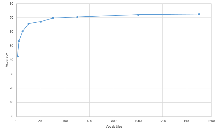
As can be seen, it is generally the case that the higher the vocab size, the higher the accuracy. However, larger vocab sizes take much longer computationally to run. A vocab size of 100 took roughly two minutes to complete, while a vocab size of 1000 took over twenty minutes to complete (4 parallel workers). The amount of improvement starts decreasing compared to the amount of time necessary for computation as the vocab size increases. This is likely because the amount of identifying clusters starts to grow too large, and that there are more clusters that stop providing as much relevant information as the original ones did. The best time and accuracy tradeoff here appears to be a vocab size of 300.
Vocabulary Feature Size Manipulation
The vocabulary feature size parameter was manipulated in this section to see what kind of an effect the size would have on the output. This pertains to the number of SIFT features used per each training image from the training set to be included into the clustering kmeans algorithm. A larger number of features results in a longer computation time for kmeans, and would most likely result in more accuracy - but the degree to which the accuracy improves is unknown. Below are the results of the manipulation. If an image did not have as many SIFT features as the number we were looking for, we simply used all the SIFT features from the image. Other parameters were kept at a constant of 300 vocab size (as determined to be the best tradeoff in the previous section), 5 step size, Fast feature calculation, and a linear SVM lambda value of 0.0001.
Displayed below is a table of the results.| Features Used | Accuracy | Results |
|---|---|---|
| 20 | 68.9% | Results |
| 50 | 68.5% | Results |
| 100 | 69.5% | Results |
| 200 | 69.3% | Results |
| 500 | 69.7% | Results |
| 1000 | 69.8% | Results |
As can be seen, it seems like the accuracy only improves at the beginning by a small amount (because if there are not enough features, the bag of SIFT features classifications will not have enough to work with and will not work as well. However, once the feature amount grows large, the amount of improvement becomes very insignificant, and is likely not worth the extra computational time. Thus, around 200 features seems to be a good tradeoff between accuracy and computation time.
Step Size Manipulation
The step size parameter was manipulated in this section to see what kind of an effect the size would have on the output. This parameter determines how many pixels to move by before extracting a SIFT descriptor. This means that if the step size is one, then all pixels in the image will be considered - this is called dense feature extraction, and is very slow computationally. A higher step size results in a faster computation time, but will lead to lower amounts of accuracy. Other parameters were kept at a constant of 300 vocab size, Fast feature calculation, 500 features for each training image for vocab size, and a linear SVM lambda value of 0.0001.
Displayed below is a table of the results.| Step Size | Accuracy | Results |
|---|---|---|
| 1 | 71.6% | Results |
| 2 | 72.3% | Results |
| 3 | 72.1% | Results |
| 4 | 69.0% | Results |
| 5 | 68.4% | Results |
| 7 | 66.7% | Results |
| 10 | 64.1% | Results |
| 15 | 58.1% | Results |
| 25 | 48.5% | Results |
| 50 | 33.3% | Results |
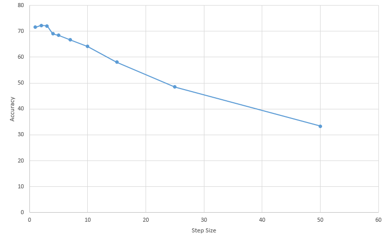
As can be seen, as the step size increases, the less accurate the results become, due to the reduce amount of SIFT features that can be used. However, as the step size increases, the computation time also decreases. A step size of one is extremely dense and takes roughly forty to fifty minutes to complete, while a step size of five takes roughly ten minutes. There was also a slight improvement from step size 1 to step size 2, likely because step size 1 may have been over-selecting features that do not accurately represent an image (such as smooth backgrounds or repetitive features).
Lambda Manipulation
The lambda parameter was manipulated in this section to see what kind of an effect the size would have on the output. Since this parameter only affects the SVM part of the pipeline, saved data from a previous run could be used to save computation time. The saved results that were used was from the run involving 300 vocab size, 500 features per trained image in the vocab section, 1 step size, and fast feature calculation.
Displayed below is a table of the results. Controlled results from a previous calculation using 0.0001 lambda had 71.6% accuracy.| Lambda Value | Accuracy | Results |
|---|---|---|
| 0.0000001 | 66.7% | Results |
| 0.000001 | 66.9% | Results |
| 0.00001 | 69.8% | Results |
| 0.00003 | 71.1% | Results |
| 0.00005 | 71.3% | Results |
| 0.00008 | 72.2% | Results |
| 0.0001 | 71.2% | Results |
| 0.001 | 64.1% | Results |
| 0.01 | 44.4% | Results |
| 0.1 | 52.7% | Results |
| 1 | 42.4% | Results |
| 10 | 45.3% | Results |
| 100 | 45.3% | Results |
As can be seen, the lambda value (regularizing parameter) seems to result in the highest accuracy at around 0.00008, which may be overfitting to this specific dataset. Values around that range all seem to be fairly consistently high.
Fast vs Not Fast
Finally, we compared the results of a Fast SIFT calculator to the results of one that did not supply the Fast parameter. This essentially doubled the run-time for this specific example (300 Vocab size, 500 features, 1 step size, 0.0001 lambda) from around fifty minutes to an hour and forty minutes. With such a small step size, however, it appears that the fast parameter does very little to improve the accuracy. The original results fell around 71.6%, but without the fast parameter, the results increased to 71.7%, which may have been just due to random chance. Results for the fast calculation can be found here, and results for the full calculation can be found here. If there were more time, additional step sizes would have been experimented with for comparison. However, due to the lengthy computation time of these results, this was not performed for this write-up.