Project 4 / Scene Recognition with Bag of Words
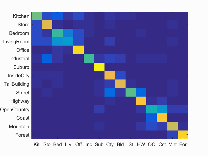
Confusion Matrix.
For features my project I implemented normalized zero mean tin image features and Bag of SIFT features. For the Bag of SIFT I implemented a standard kmeans 200 word vocabulary, but I also implemented a Fisher features using a Gaussian Mixture Model. In addition to that I added the calculation of a GIST feature to the final Fisher feature to further improve accuracy. Finally I also use 15 linear SVM classifiers to do a more accurate classification of the categories. The rest of the write up will be organized in the following way:
- Tiny Image features
- Nearest Neighbor classifier
- Bag of SIFT features
- Linear SVM classifier
- Results
Tiny Image features
My implementation of Tiny image features is fairy standard as I just use imresize to shrink the image to a 16x16 patch. However, I also change the 256 dimension array to be zero mean and then normalized it. This improved accuracy from 19.1% to 22.5%.
Nearest Neighbor classifier
My implementation of the Nearest neighbor classifier was simple as well. I simply used vl_alldist2 and min to find the 1 nearest neighbor. I only did 1-NN as I was already getting 22.5% accuracy with Tiny Images and 52.3% accuracy with Bag of SIFT.
Bag of SIFT features
My implementation of the Bag of SIFT features was more complicated. I have two versions of my implementation. One version uses vl_kmeans to create a 200 word vocabulary that I use vl_alldist2 to match features to. This is for use with the 1-NN classifier as the other version has such a high dimension it makes 1-NN too slow and inaccurate. The other version is to use vl_gmm to create a Gaussian Mixture Model for use in creating a Fisher encoding vector. After constructing the fisher vector I also create a GIST feature for the image using the code linked to in the assignment description. The code for my Bag of SIFT is below:
for i = 1 : dim(1)
    % read image
    img = imread(char(image_paths(i)));
    gray = single(mat2gray(img));
    % make SIFT features
    [locations, SIFT_features] = vl_dsift(gray, 'step', 10, 'fast');
    if(fisher)
        encoding =  vl_fisher(single(SIFT_features), MEANS, COVARIANCES, PRIORS, 'Normalized');
        [gist, p] = LMgist(img, '', param);
        ret(i,1 : 51200) = encoding(:);
        ret(i, 51201: 51208) = gist';
    else
        dist = vl_alldist2(vocab, single(SIFT_features));
        [confidence, index] = min(dist);
        hist = zeros(1, vocab_size);
        for j = 1 : size(SIFT_features, 2)
           hist(1,index(j)) = hist(1,index(j)) + 1;
        end
        hist = hist/norm(hist(:));
        ret(i,:) = hist(:);
    end
end
When adding the Fisher encoding and GIST feature my accuracy jumped from 59.1% to 70.3%.
Linear SVM classifier
My implentation of the linear SVM classifier was also fairly standard. I run vl_svmtrain 15 times to train SVMs for each category. To optimize the code, instead of immeadiatly running the trained SVM on the images I instead train all 15 SVM and save their learned parameters in an array. I then run all 15 SVMs on each image picking the maximally responding SVM as the category for that image. The code for saving all of the SVMs in an array is shown below:
s = size(train_image_feats, 2)+ 1;
svms = zeros(num_categories, s);
for i = 1 : num_categories
    labels = double(strcmp(categories(i), train_labels));
    labels(labels == 0) = -1;
    [W B] = vl_svmtrain(train_image_feats', labels', 0.00001);
    svms(i, 1) = B;
    svms(i, 2:s) = W;
end
Results
| Type | Accuracy | Total time | Time for features | Time for classifier |
|---|---|---|---|---|
| Tiny Image - 1-NN | 22.5% | 18.9374 sec | 13.2347 sec | 5.7027 sec |
| Bag of SIFT - 1-NN | 52.3% | 3.5165 min | 3.43196667 min | 4.99244 sec |
| Bag of SIFT - Lin. SVM | 70.3% | 7.61695 min | 6.67193333 min | 56.7012 sec |
Below are the results of the final Bag of sift feature - SVM classifier run.
Scene classification results visualization
Accuracy (mean of diagonal of confusion matrix) is 0.703
| Category name | Accuracy | Sample training images | Sample true positives | False positives with true label | False negatives with wrong predicted label | ||||
|---|---|---|---|---|---|---|---|---|---|
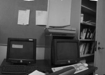
| Kitchen | 0.580 |  |
 |
 |
 |
 TallBuilding |
 Bedroom |
 Office |
 Bedroom |
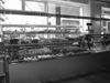
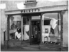
| Store | 0.770 | 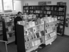 |
 |
 |
 |
 Kitchen |
 Industrial |
 InsideCity |
 Industrial |
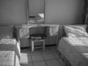
| Bedroom | 0.500 |  |
 |
 |
 |
 LivingRoom |
 LivingRoom |
 LivingRoom |
 LivingRoom |
| LivingRoom | 0.340 |  |
 |
 |
 |
Bedroom |
 Bedroom |
 Industrial |
 Office |
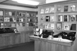
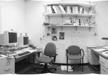
| Office | 0.920 |  |
 |
 |
 |
 Bedroom |
 Store |
 Bedroom |
 LivingRoom |
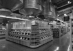
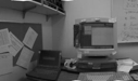
| Industrial | 0.530 | 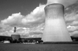 |
 |
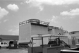 |
 |
LivingRoom |
Store |
 Store |
 TallBuilding |
| Suburb | 0.980 |  |
 |
 |
 |
 Coast |
 OpenCountry |
 TallBuilding |
 Store |
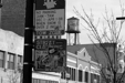
| InsideCity | 0.800 |  |
 |
 |
 |
 Highway |
 Street |
 Bedroom |
 TallBuilding |
| TallBuilding | 0.780 |  |
 |
 |
 |
 InsideCity |
Suburb |
 InsideCity |
 Highway |
| Street | 0.560 |  |
 |
 |
 |
 Forest |
 Coast |
 Highway |
 Store |
| Highway | 0.850 |  |
 |
 |
 |
 Street |
 Street |
 Forest |
 LivingRoom |
| OpenCountry | 0.450 |  |
 |
 |
 |
 Mountain |
 Coast |
 Suburb |
 Coast |
| Coast | 0.860 |  |
 |
 |
 |
 Mountain |
 OpenCountry |
 OpenCountry |
| Mountain | 0.730 |  |
 |
 |
 |
 Coast |
 Forest |
 OpenCountry |
 OpenCountry |
| Forest | 0.900 |  |
 |
 |
 |
 Mountain |
 OpenCountry |
 Store |
 Mountain |
| Category name | Accuracy | Sample training images | Sample true positives | False positives with true label | False negatives with wrong predicted label | ||||