Example of a right floating element.

Tiny KNN: 22%

Tiny Images + K-NN

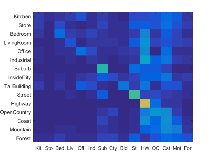
Our first way to represent an image descriptor was using tiny images. The images were all scaled down to a 16x16 pixel image. This is a basic image descriptor that captures an image's general intensity layout since each pixel on the tiny image represents multiple images on the original image. With this descriptor we then classified the training set using K-NN. Nearest neighbor was very simple in that it just finds the K nearest training neighbors in the feature space. Implementing these two algorithms were trivial and they didn't produce good accuracies (18% - 21%). This could be the case because the image descriptor was very poor and only focused on pixel intensities. Using this descriptor doesn't hold many properties such as high or low frequencies and spatial features.

        function image_feats = get_tiny_images(image_paths)
        % image_paths is an N x 1 cell array of strings where each string is an
        %  image path on the file system.
        % image_feats is an N x d matrix of resized and then vectorized tiny
        %  images. E.g. if the images are resized to 16x16, d would equal 256.

        image_size = size(image_paths, 1);
        d = 16;

        image_feats = zeros(image_size, d*d);
        for p = 1:image_size
            path = image_paths{p};
            image = imread(path);
            small_image = double(reshape(imresize(image, [d, d]), [1, d*d]));
            small_image = small_image - mean(small_image);
            small_image = small_image/norm(small_image);
            image_feats(p,:) = small_image;
        end

        end   
            

        function predicted_categories = nearest_neighbor_classify(train_image_feats, train_labels, test_image_feats)
        % train_image_feats is an N x d matrix, where d is the dimensionality of the
        %  feature representation.
        % train_labels is an N x 1 cell array, where each entry is a string
        %  indicating the ground truth category for each training image.
        % test_image_feats is an M x d matrix, where d is the dimensionality of the
        %  feature representation. You can assume M = N unless you've modified the
        %  starter code.
        % predicted_categories is an M x 1 cell array, where each entry is a string
        %  indicating the predicted category for each test image.

        k = 15;
        [test_size, ~] = size(test_image_feats);
        d_matrix = vl_alldist2(test_image_feats', train_image_feats');
        predicted_categories = cell(test_size, 1);

        [~, index] = sort(d_matrix, 2);

        for r = 1:test_size
            k_labels = train_labels(index(r, 1:k))';
            
            [unique_labels, ~, ic] = unique(k_labels, 'stable');
            mode_label = unique_labels(mode(ic));
            predicted_categories{r, 1} = string(mode_label);
            
        end

        end
            

Bag of Feats KNN: 60%

Bag of Features + K-NN

Before implementing bag of SIFTs, we had to create a vocabulary dictionary of features. How we did this was by sampling training images for SIFT features and then performing KMeans on all the features to get K clusters. Our vocabulary size was default to 200. I also decided to use the KD-tree which improved time complexity and also incresed my accuracy by about 7%

Implementing bag of features was pretty straight forward. Using our vocabular dictionary of features, for each image in our training set we would find many SIFT descriptors. We would then create a histogram of width vocab_size (each vocab feature has it's own bin) and for each SIFT descriptor we would find which vocab feature it most resembled (distance) and increment the respective vocab feature's bin. This would create a histogram of width vocab size where all the bars would sum to the number of image SIFT descriptors. This histogram would be the image's descriptor. This image descriptor works better than the tiny image because it takes into account the vocab dictionary. The vocab would theoretically take common SIFT features from categories such as a refrigerator handle or ocean waves or anything else specific to scenes. So when we make our image feature we may get bins that have more scenic features. When we then do classification, the test images and training images would have similar distributions of bins. This idea weakens if the vocab dictionary includes generic sift features such as a brick wall or table corner since other scenes may include this. One way to do better could be to sample more characteristic images to create the vocab dictionary.

I also included the spacial pyramid feature with only 2 levels. This increased my accuracy by 3-4% since bag of features loses spacial representation of features. With 2 levels and a vocab size of 200 each image descriptor was 1000 dimensions wide. Later when doing Bag of Features and SVM, 2 levels gave me 73% while 3 levels gave me 78%, but I stuck to 2 levels because 3 levels takes a long time to compute.

Bag of Features

        function image_feats = get_bags_of_sifts(image_paths)
        % image_paths is an N x 1 cell array of strings where each string is an
        % image path on the file system.

        step = 10;

        load('vocab.mat')
        [vocab_size, vocab_d] = size(vocab);
        [image_size, taeyeon] = size(image_paths);
        image_feats = zeros(image_size, vocab_size);

        % for each image
        for p = 1:image_size
            path = image_paths{p};
            image = imread(path);
            image = gaussian_image(image, 0);
            image = im2single(image);

            % find image sift features of d = 128
            [locations, sift_features] = vl_dsift(image, 'fast', 'step', step);
            sift_features = single(sift_features'); % F x d
            
            % for each sift_feature, find closest vocab feature
            % distance matrix of each sift_feature to each vocab centroid
            % sort each row: sift_feature(x, 1) index is vocab index
            d_matrix = vl_alldist2(sift_features', vocab');
            [sorted_d_matrix, index] = sort(d_matrix, 2);
            index = index(:, 1)';
            
            % for each index, increment image_feature row at that index
            % each row index has dimension size(vocab)
            for r = 1:size(sift_features, 1)
                image_feats(p, index(r)) = image_feats(p, index(r)) + 1;
            end
            
            % normalize
            image_feats(p, :) = image_feats(p, :)/norm(image_feats(p, :));
        end

            

Bag of Features with spacial pyramid

        function image_feats = get_bags_of_sifts(image_paths)

        levels = 2;

        step = 5;

        load('vocab.mat');
        [vocab_size, vocab_d] = size(vocab);
        [image_size, taeyeon] = size(image_paths);
        image_feats = zeros(image_size, uint32(vocab_size/3*(4 .^ levels - 1)));

        forest = vl_kdtreebuild(vocab');

        % for each image
        for p = 1:image_size
            path = image_paths{p};
            image = imread(path);
            image = gaussian_image(image, 0);
            image = im2single(image);

            [image_h, image_w] = size(image);
            % find image sift features of d = 128
            [locations, sift_features] = vl_dsift(image, 'fast', 'step', step);
            sift_features = single(sift_features'); % F x d
            
            image_feature = [];
            for l = 0:(levels - 1)
                % Number of cells wide
                cells_wide = 2 .^ l;
                c_width = image_w / cells_wide;
                c_height = image_h / cells_wide;
                
                % For each cell top left corner
                for r = 0:cells_wide - 1
                    for c = 0:cells_wide - 1
                        % Finding window of features based on level and grid
                        % TL, TR, BR, BL clockwise
                        xv = [c*c_width, (c+1)*c_width, (c+1)*c_width,(c)*c_width];
                        yv = [r*c_height, r*c_height, (r+1)*c_height, (r+1)*c_height];
                        xq = locations(1, :);
                        yq = locations(2, :);

                        inside_locations = inpolygon(xq,yq,xv,yv);
                        inside_feats = sift_features(inside_locations > 0, :);
                                        
                        % Using forest, index is 1 x size(sift_features) 
                        [index, ~] = vl_kdtreequery(forest, vocab', inside_feats', 'NumNeighbors', 3);

                        % Making histogram
                        level_cell_feats = zeros(1, vocab_size);
                        for i = 1:vocab_size
                            level_cell_feats(1, i) = sum(index(:) == i);
                        end
                        
                        image_feature = [image_feature level_cell_feats];
                    end
                end    
                image_feature = image_feature/(2 .^ (levels - 1 - l));
            end
            % normalize
            image_feats(p, :) = image_feature/norm(image_feature);
        end



            

Vocab Size Extra Credit

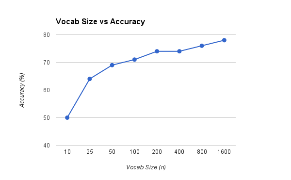
I attempted to analyze how our main project would be affected by a different vocab size. We would imagine that a small vocab size would not maintain enough features to appear in all the different types of images and categories being labeled. However having a too large vocab size may overfit our data since we only have hundreds of images per category which doesn't represent the entire category space. In our example we took vocab sizes of 10, 25, 50, 100, 200, 400, 800, and 1600. There was a significant increase from 10 to 25 and 100 to 200 and overall caps at around 75% accuracy with no more significant increase with larger vocab size. With an increase in vocab size we fall into overfitting our training set which doesn't help in looking at other test data.

Vocab Sizes vs Comparisons

Vocab size vs. accuracy. On hover: (vocab size - accuracy)

Vocab Dictionary

        function vocab = build_vocabulary( image_paths, vocab_size )
        % The inputs are 'image_paths', a N x 1 cell array of image paths, and
        % 'vocab_size' the size of the vocabulary.
        % The output 'vocab' should be vocab_size x 128. Each row is a cluster
        % centroid / visual word.


        [image_size, taeyeon] = size(image_paths);
        features = zeros(128, 0);
        step = 25;

        % Find sift features for each training image
        for p = 1:image_size
            path = image_paths{p};
            image = imread(path);
            image = gaussian_image(image, 0);
            image = im2single(image);

            [locations, sift_features] = vl_dsift(image, 'fast', 'step', step);
            
            % Append new sift features
            features = [features, sift_features];
        end

        % Perform KMeans to find vocab_size centroids
        sift_features = single(features);
        [vocab, assignments] = vl_kmeans(sift_features, vocab_size);
        vocab = vocab';

        end
            

Bag of Feats SVM: 73%

Bag of Features + SVM

This section we used an SVM classifier instead of KNN. KNN has trouble because it's hard to get the correct K value which determines the influences of both near and far neighbors. SVM could do a better job through creating hyper planes to distingush scenes. If all images of a certain category have lots of SIFT descriptors of water or kitchen utensils, then it would be easier to seperate images with and without this descriptors (if they are uniquly characteristic to the scene). What we did was create 1 vs all SVMs for every category, trained each SVM to get a dimension weights (hyperplane), plugged in the test descriptor's values into the hyperplane function, and see what the value is (+ or -). We took the SVM value that was most positive and assigned the image with that SVM's category. I ended up with a lambda value of 0.00005 through trying multiple values.

SVM

        function predicted_categories = svm_classify(train_image_feats, train_labels, test_image_feats)
        % image_feats is an N x d matrix, where d is the dimensionality of the
        %  feature representation.
        % train_labels is an N x 1 cell array, where each entry is a string
        %  indicating the ground truth category for each training image.
        % test_image_feats is an M x d matrix, where d is the dimensionality of the
        %  feature representation. You can assume M = N unless you've modified the
        %  starter code.
        % predicted_categories is an M x 1 cell array, where each entry is a string
        %  indicating the predicted category for each test image.

        lambda = 0.00005;
        categories = unique(train_labels); 
        num_categories = length(categories);

        svm = cell(num_categories, 2);

        % Creating 1 vs all SVMs
        for c = 1:num_categories
            category = categories{c};
            labels = strcmp(category, train_labels) * 2 - 1;
            [W B] = vl_svmtrain(train_image_feats', labels', lambda);
            svm{c, 1} = W;
            svm{c, 2} = B;
        end

        test_size = size(test_image_feats, 1);
        predicted_categories = cell(test_size, 1);

        % For each test image, find the SVM which gives the most positive number
        %   indicating which side of the hyperplane the test_image_feat was on.
        %   The svm that produces the highest value uses it's category.
        for i = 1:test_size
            image_feat = test_image_feats(i, :);
            W = svm{1, 1};
            B = svm{1, 2};
            max_category = categories{1};
            max = W' * image_feat' + B;
            for c = 2:num_categories
                W = svm{c, 1};
                B = svm{c, 2};
                category = categories{c};
                val = W' * image_feat' + B;
                if val > max
                    max_category = category;
                    max = val;
                end
            end
            
            predicted_categories{i, 1} = max_category;
        end

            

Gaussians Bag of Sifts

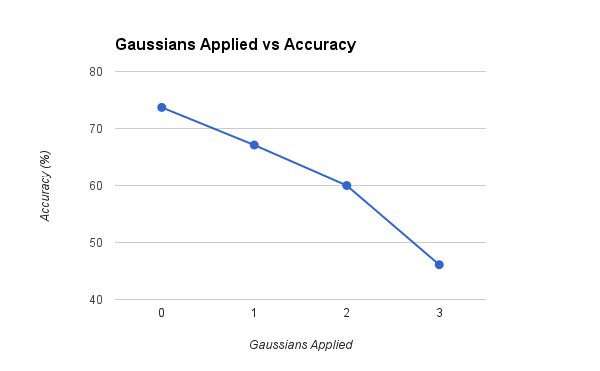
We experimented in the bag of sifts section by smoothing and sampling images before running them through the algorithms. We performed this step for 4 levels (0 - 3) of the gaussian pyramid to see how well these images would affect the accuracy of the algorithm. We can see that the more gaussian smoothing applied the worse accuracy we get. I think with more smoothing and sampling applied, the SIFT descriptors of the image get harder to find, so fine details specific to certain scenes may be lost or generalized to match other generalized SIFT descriptors on other scenes. Applying this method seems to not benifit the algorithm.

Gaussian Sampling

        % This code will take an image and scale it based on the gaussian pyramid.
        function ret_image = gaussian_image(image, level)
            ret_image = image;
            while level > 0
                ret_image = impyramid(ret_image, 'reduce');
                level = level - 1;
            end
        end
            

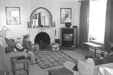
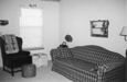
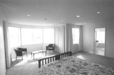
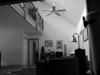
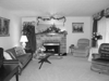
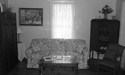
Scene classification results visualization

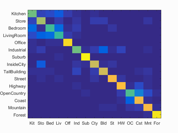
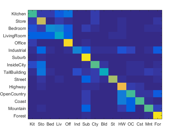
Accuracy (mean of diagonal of confusion matrix) is 0.730

Category name	Accuracy	Sample training images		Sample true positives		False positives with true label		False negatives with wrong predicted label
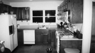
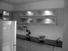
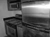
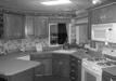
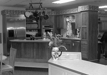
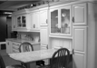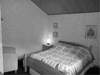
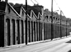
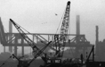
Kitchen	0.580					Bedroom	Industrial	LivingRoom	LivingRoom
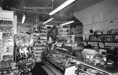
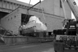
Store	0.670					Industrial	LivingRoom	TallBuilding	Kitchen
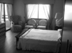
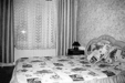
Bedroom	0.520					LivingRoom	LivingRoom	LivingRoom	TallBuilding
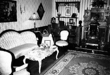
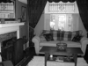
LivingRoom	0.510		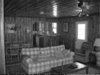			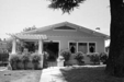Suburb	Kitchen	Kitchen	Store
Office	0.910					Bedroom	Kitchen	Street	InsideCity
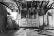
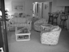
Industrial	0.580					Bedroom	InsideCity	TallBuilding	InsideCity
Suburb	0.970					OpenCountry	LivingRoom	LivingRoom	Store
InsideCity	0.720					Kitchen	Industrial	Kitchen	Industrial
TallBuilding	0.740					Industrial	Mountain	Industrial	Coast
Street	0.820					Bedroom	Mountain	Store	Mountain
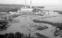
Highway	0.830					Industrial	Industrial	InsideCity	Coast
OpenCountry	0.540					Mountain	Coast	Highway	Coast
Coast	0.800					OpenCountry	Highway	OpenCountry	Mountain
Mountain	0.820					Store	OpenCountry	Coast	Coast
Forest	0.940					Mountain	Mountain	Mountain	Mountain
Category name	Accuracy	Sample training images		Sample true positives		False positives with true label		False negatives with wrong predicted label