Project 4 / Scene Recognition with Bag of Words

In this project we mainly perform scene recognition with Bag of Sift features and linear SVM classifiers. Bag of Features is analogous to Bag of Words which is widely used in natual language processing. It dominated the recognition task for the past decade before deep learning emerged. Algorithm will be detailed later on.

In order to show the robustness of the combination of BoF and SVM, we compare these three approaches:

1. tiny image feature with nearest neighbor (NN) classifier (obtains 22.5% accuracy)
2. bag of sifts feature with NN classifier (obtains 50.3% accuracy)
3. bag of sifts feature with SVM classifier (obtains 64.4% accuracy)

1. Tiny image feature with NN classifier

Tiny image feature simply resizes images to a certain size (16 by 16), vectorizes it to obtain the 256-d feature. It is not robust, but can give us a basic idea.

We use 1-NN here. Both training data and test data have size of 1500 in our experiemnts. For each test data, we look for the training data that has the nearest distance with it in the feature space, and label the test data with the label of the training data.

Results of tiny image feature with 1-NN:

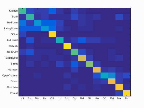
Accuracy (mean of diagonal of confusion matrix) is 0.225

Category name	Accuracy	Sample training images		Sample true positives		False positives with true label		False negatives with wrong predicted label
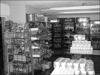
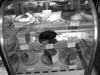
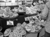
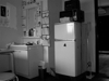
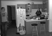
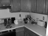
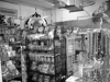
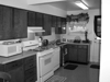
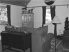
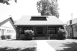
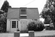
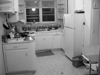
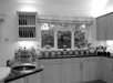
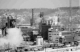
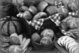
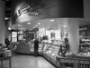
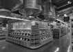
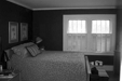
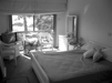
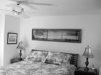
Kitchen	0.080					Store	Bedroom	Store	TallBuilding
Store	0.020		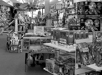			Forest	Forest	OpenCountry	Coast
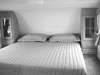
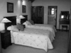
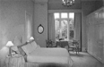
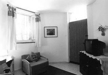
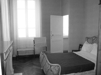
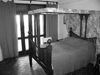
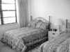
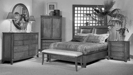
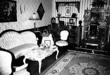
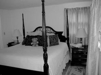
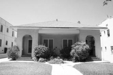
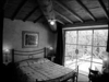
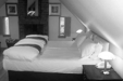
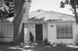
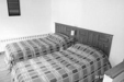
Bedroom	0.180		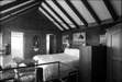			OpenCountry	Street	Coast	Kitchen
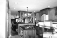
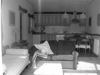
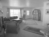
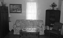
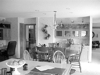
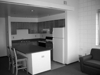
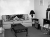
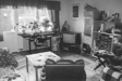
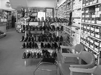
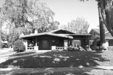
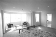
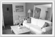
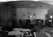
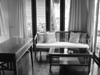
LivingRoom	0.100					Suburb	Store	Bedroom	Highway
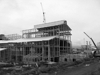
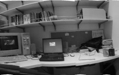
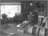
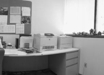
Office	0.180		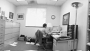			Street	InsideCity	Highway	Industrial
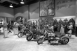
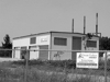
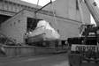
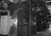
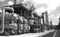
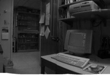
Industrial	0.130					Bedroom	Bedroom	Forest	Highway
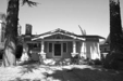
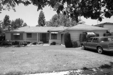
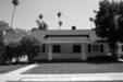
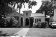
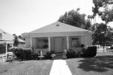
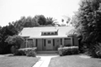
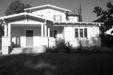
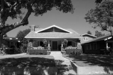
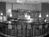
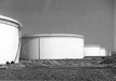
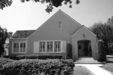
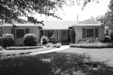
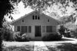
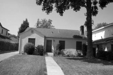
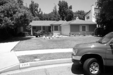
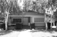
Suburb	0.370		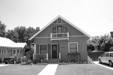			Street	Office	Industrial	TallBuilding
InsideCity	0.060					Store	Store	Mountain	OpenCountry
TallBuilding	0.220					Kitchen	Kitchen	Highway	Office
Street	0.420					Mountain	LivingRoom	InsideCity	Mountain
Highway	0.560					Coast	Suburb	OpenCountry	OpenCountry
OpenCountry	0.350					Kitchen	Suburb	Highway	Bedroom
Coast	0.390					Store	OpenCountry	OpenCountry	Suburb
Mountain	0.180					Forest	LivingRoom	Street	Highway
Forest	0.130					InsideCity	InsideCity	Kitchen	InsideCity
Category name	Accuracy	Sample training images		Sample true positives		False positives with true label		False negatives with wrong predicted label

2. BoF with NN classifier

We first build vocabulary of Sifts from training set. We extract dense Sift features using vlfeat function with a step size of 10, and sample a total of 50k Sift features from the whole training set. Then we use kmeans to cluster them into 200 vocabularies.

To save memory, we sample the same number of features from each training image, and only put them into the sampled_feat matrix:

N = length(image_paths);
sample_per_train_im = floor(k/N);
k = sample_per_train_im * N;
sampled_feat = zeros(feat_dim, k);

for i=1:N
  im = imread(image_paths{i});
  im = im2single(im);
  [locations, SIFT_features] = vl_dsift(im, 'step', step ,'fast');
  num_sift = size(SIFT_features, 2);
  sample_idx = randi(num_sift, sample_per_train_im, 1);
  sample_sift = SIFT_features(:, sample_idx);
  sampled_feat(:, (i-1)*sample_per_train_im+1 : i*sample_per_train_im) = sample_sift;
end

Then we compute bag of sifts for both training images and test images. For each input image, we extract dense sift features with a step of 7 (denser than when we build vocalubary because we only need cluster centroid, but now we need more precise descriptions of each image to build feature), find the nearest vocabulary center for each feature, and build a histogram (counting the frequency that each vocabulary appears in an image). Note that each histogram is L1-normalized to make sure the BoF of each image is comparable.

N = length(image_paths);
image_feats = zeros(N, vocab_size);

for i=1:N
  hist_i = zeros(1,vocab_size);
  im = imread(image_paths{i});
  im = im2single(im);
  [locations, SIFT_features] = vl_dsift(im, 'step', step, 'fast');
  num_sift = size(SIFT_features, 2);

  dist = vl_alldist2(single(SIFT_features), vocab');
  [min_train, min_idx] = min(dist, [], 2); % return column vectors % min_idx ranges from 1 to vocab_size
  hist_i = hist(min_idx, 1:vocab_size); % 1 x vocab_size
  hist_i = hist_i / sum(hist_i);
  image_feats(i,:) = hist_i;
end

We still use 1-NN as classifier. The performances rises to over 50%, showing that BoF is robust in scene recognition.

Results of bag of sifts feature with 1-NN classifier:

Accuracy (mean of diagonal of confusion matrix) is 0.503

Category name	Accuracy	Sample training images		Sample true positives		False positives with true label		False negatives with wrong predicted label
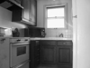
Kitchen	0.390		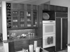			Office	LivingRoom	Store	Office
Store	0.420					Industrial	Industrial	Street	Industrial
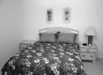
Bedroom	0.220		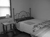			Suburb	Kitchen	LivingRoom	Kitchen
LivingRoom	0.330					Bedroom	TallBuilding	Industrial	Kitchen
Office	0.750					Bedroom	Store	Bedroom	Kitchen
Industrial	0.340					Store	InsideCity	Street	Street
Suburb	0.870		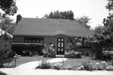			Street	Highway	Street	TallBuilding
InsideCity	0.330					Street	Street	Kitchen	Street
TallBuilding	0.270					Kitchen	Bedroom	Industrial	LivingRoom
Street	0.520					Store	LivingRoom	Industrial	Kitchen
Highway	0.730					Coast	OpenCountry	Street	Suburb
OpenCountry	0.430					Coast	Mountain	Suburb	Coast
Coast	0.500					OpenCountry	OpenCountry	Highway	Highway
Mountain	0.560					TallBuilding	TallBuilding	Highway	Forest
Forest	0.880					OpenCountry	TallBuilding	OpenCountry	Mountain
Category name	Accuracy	Sample training images		Sample true positives		False positives with true label		False negatives with wrong predicted label

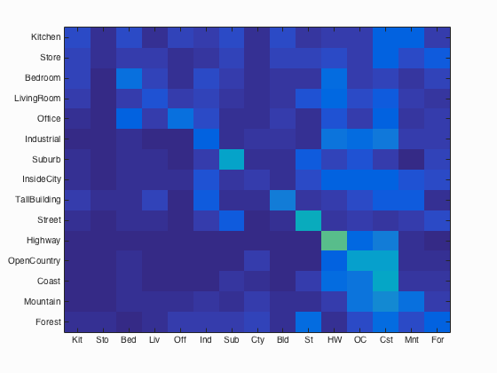
3. BoF with linear SVM classifier

Support Vector Machines (SVM) had been the state-of-the-art classifier before deep learning showed up. Here we use a simple linear SVM. We train SVM for each category, finding a liner hyperplane in feature space that best separates positive and negative samples.

Then we use the resulted weight and bias, multiply and add them back to test images. A higher number means the test sample is closer to this category, so we compare the score of a test image for each category classifiers, and classify this image into the category that has the highest score.

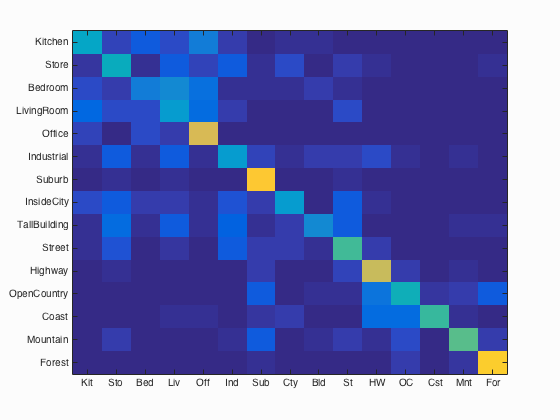
With the regularization parameter LAMBDA of 0.000004 gave us a classification accuracy of 64.4%, which shows the robustness of the combination of bag of sifts feature and SVM classifier.

for i=1:num_categories
  name_cat = categories{i};
  pos_train_idx = strcmp(name_cat, train_labels);
  binary_labels = -1 * ones(1, num_test_images);
  binary_labels(pos_train_idx) = 1;
  [W, B] = vl_svmtrain(train_image_feats', double(binary_labels), LAMBDA);
  test_scores = W'*test_image_feats' + B;
  % test_image_feats' - d x N
  % W - d x 1
  % B - 1 x N (?)
  % test_scores - 1 x N

  test_scores_matrix(i,:) = test_scores;
end

[~, test_labels_numeric] = max(test_scores_matrix);

Bag of sifts feature with SVM classifier:

Accuracy (mean of diagonal of confusion matrix) is 0.644

Category name	Accuracy	Sample training images		Sample true positives		False positives with true label		False negatives with wrong predicted label
Kitchen	0.530		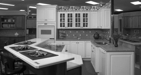			LivingRoom	Office	Office	Office
Store	0.500		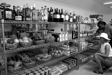			Industrial	Bedroom	Kitchen	Mountain
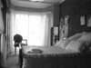
Bedroom	0.320		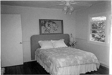			LivingRoom	Kitchen	Office	Kitchen
LivingRoom	0.320		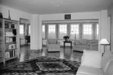			Bedroom	Industrial	Store	Office
Office	0.910					TallBuilding	LivingRoom	Kitchen	Kitchen
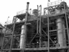
Industrial	0.450					LivingRoom	Highway	TallBuilding	Store
Suburb	0.940		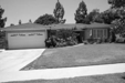			Industrial	Industrial	InsideCity	InsideCity
InsideCity	0.560					Highway	Street	Store	TallBuilding
TallBuilding	0.740					Store	LivingRoom	Mountain	InsideCity
Street	0.610					Forest	Industrial	Industrial	Suburb
Highway	0.790					OpenCountry	OpenCountry	InsideCity	Coast
OpenCountry	0.400					Highway	Coast	Coast	Mountain
Coast	0.810					OpenCountry	OpenCountry	Mountain	Highway
Mountain	0.860					Store	Bedroom	Suburb	TallBuilding
Forest	0.920					OpenCountry	OpenCountry	Mountain	Mountain
Category name	Accuracy	Sample training images		Sample true positives		False positives with true label		False negatives with wrong predicted label