Project 4 / Scene Recognition with Bag of Words
The purpose of this project is to perform basic image recognition with tiny images and bags of quantized local features as features into classification algorithms, specifically k-nearest neighbors and linear support vector machines. We will attempt to classify scenes into one of 15 categories by training and testing on 15 scene database deriving from Lazebnik et al. 2006. Project is divided into three sections.
- Tiny images representation and nearest neighbor classifier
- Bag of SIFT representation and nearest neighbor classifier
- Bag of SIFT representation and linear SVM classifier
Tiny images representation and nearest neighbor classifier
Tiny image feature works by downscaling the image to a fixed resolution, in which I've reduced each image to 16x16 pixels. I also performed feature scaling standardization (zero mean and unit length) to increase the classification performance. While simple and quick to compute, tiny images do not work well, because we are neglecting high frequencies and spatial or brightness shifts. With the features calculated, we prepare training and testing samples to k-nearest neighbors classification algorithm. Each testing example is labeled with its k-nearest training samples with corresponding labels. In the case of multiple class match with same most counts with k > 1 samples (ties), I pick the class that matlab's 'mode' function picks (; however, I should pick the closest of multiple matches). 'vl_alldist2' method was used for calculating the distances for finding nearest points.
Without normalizatrion, 1NN accuracy with tiny image features is 0.194. With normalization, 1NN accuracy becomes 0.224. This is likely, because KNN (k-nearest neighbors) algorithm calculates distance between two points with some distance function, usually Euclidean distance. Some image features may have broad range of values.
Now, we try different k values for KNN.
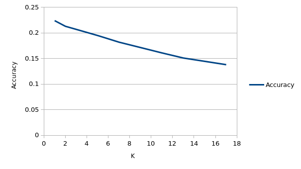
At K = 1, accuracy is 0.224, but at K = 67, accuracy is 0.071 which is close to random chance. Generally, we reduce wrong classification due to noise by increasing K, but it appears that many features overlap with different classes and we'd rather choose a single point that is closest to training examples.
Bag of SIFT representation and nearest neighbor classifier
For bag of SIFT representation, we will be using SIFT to find features for our images, but will have few intermediate steps. We first set up a 'vocabulary' of 'words' that describe an image, and set the frequencies of these words as features. Vocabulary is setup by taking SIFT features of all images, and clustering them to x number of words. I used k-means clustering algorithm which clusters data through separating samples in x groups of equal variance. The means of each x groups or clusters are called centroids, and x is again equivalent to number of words in our vocabulary. Centroids are saved In the vocabulary to see what SIFT features fit most well with these words. After setting up our vocabulary, we obtain SIFT features again for each image but we check the centroids and count the number of words (from vocabulary) that show up. Each word in vocabulary will become our feature, and corresponding values will be the number of matched words appeared for a particular image.
I chose parameters as below, and I will explain the reasoning in the third part.
binSize = 3; % SIFT bin size
stepSize = 8; % SIFT step size (build_vocabulary)
stepSize = 4; % SIFT step size (get_bags_of_sifts)
vocab_size = 400;
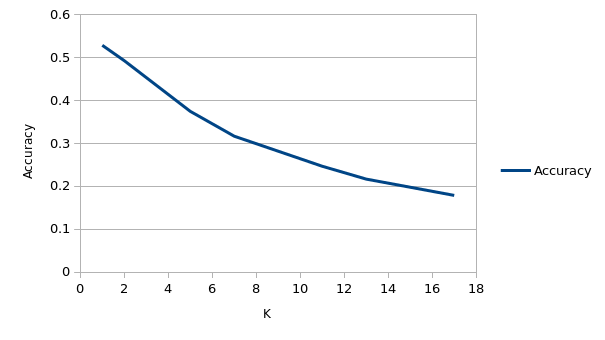
At K = 1, accuracy is 0.529, and at K = 17, accuracy is 0.179. 1NN gives low bias but gives high variance. We are validating our accuracies through 50/50 split rather than through X fold cross validation. Thus, 1NN may not be the best option. However, we will trust our 50/50 split test. Note: 2NN accuracy (0.493) is not far from 1NN.
Bag of SIFT representation and linear SVM classifier
We will be using linear SVM classifier for this project although there are multiple kernels we can employ. There are also two types of SVMs for multiclass supervised learning, and we will be using 1-vs-all method where we construct our dataset in a way that we run multiple binary SVM classification with one scene (class value = '1') against all other scenes ('-1').
For bag of SIFT representation, accuracy did not improve much with small varying bin and step sizes. With smaller step size, performance tended to improve slightly with huge time penalty. However, keeping step size for building vocabulary larger than step size at assigning feature values showed noticeable accuracy improvements. Resulting bin size was 3 as method default value, and step sizes were 8 and 4 respectively.
For speed optimization, KD-trees was used for finding nearest points, and 100 randomly sampled SIFT features per image was used to build the vocabulary.
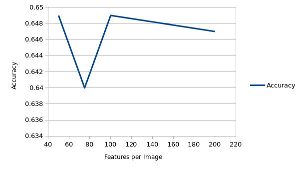
Interestingly, randomly sampling SIFT features helped to improve accuracy as 100 features per image gave 0.649 accuracy with lambda at 1e-6 and vocab size at 400, compared to 0.621 at no random sampling. However, note that we are randomly sampling features, and scores may change based on different runs and from cross validation.
Increasing vocabulary size generally increased the accuracy to a certain point.
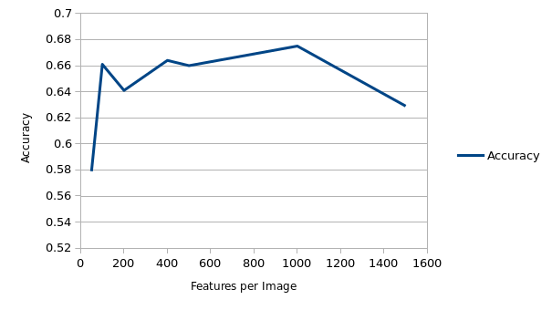
I chose vocabulary size of 400 based on speed and accuracy improvements.
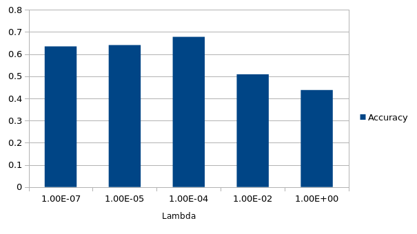
Modifying lambda for SVM caused large variation in accuracies, but I was able to capture a local maxima at 1e-4.
Normalizing features did not improve the accuracy (Not sure if it was done right).
Extra credit: TreeBagger (Random Forest) classifer
I've tried an additional classification algorithm, random forest (ensemble of decision trees) with bootstrap aggregating. With increase in number of weak learners, the accuracy increased as expected. But higher number came with higher computational penalty.
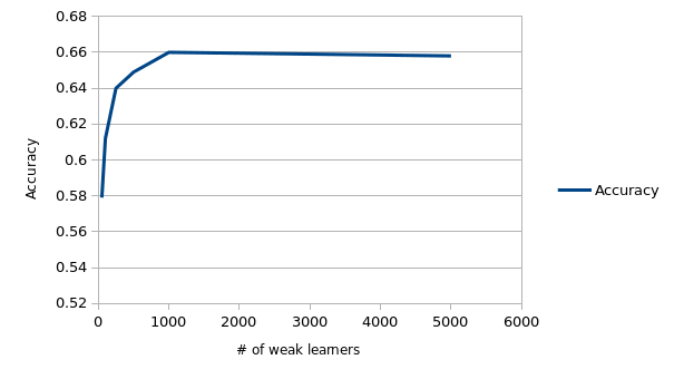
The accuracy was comparable with the SVM. Also, small number of weak learners, like 250, was very quick.
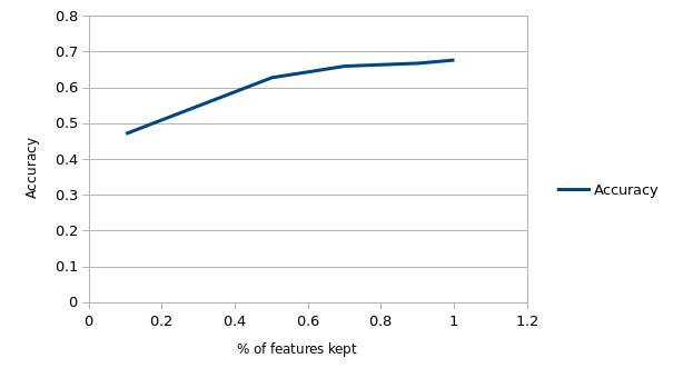
Extra credit: Entropy based feature selection
With random forest, I've also tried classification with feature selection. The results of entropy based feature selection is shown below.
Best performer
binSize = 3; % SIFT bin size
stepSize = 8; % SIFT step size (build_vocabulary)
stepSize = 4; % SIFT step size (get_bags_of_sifts)
vocab_size = 400;
LAMBDA = 1e-4; % SVM lambda value
featuresPerImg = 100; % # of randomly sampled SIFT features per image
Scene classification results visualization

Accuracy (mean of diagonal of confusion matrix) is 0.678
| Category name | Accuracy | Sample training images | Sample true positives | False positives with true label | False negatives with wrong predicted label | ||||
|---|---|---|---|---|---|---|---|---|---|
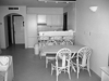
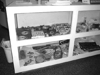
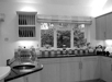
| Kitchen | 0.580 |  |
 |
 |
 |
 Bedroom |
 Store |
 TallBuilding |
 LivingRoom |
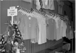
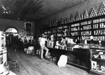
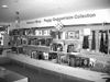
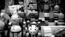
| Store | 0.650 | 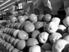 |
 |
 |
 |
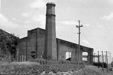
 Industrial |
 Bedroom |
 Kitchen |
 LivingRoom |
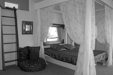
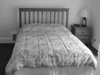
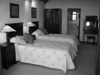
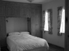
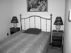
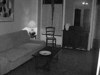
| Bedroom | 0.350 |  |
 |
 |
 |
 Kitchen |
 Industrial |
 Store |
 Office |
| LivingRoom | 0.350 |  |
 |
 |
 |
 Industrial |
 Store |
 Bedroom |
 Kitchen |
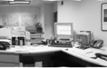
| Office | 0.910 | 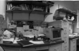 |
 |
 |
 |
 Store |
 LivingRoom |
 LivingRoom |
 Bedroom |
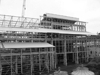
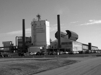
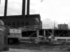
| Industrial | 0.580 | 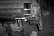 |
 |
 |
 |
 TallBuilding |
 InsideCity |
 Forest |
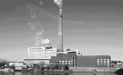 InsideCity |
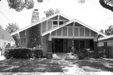
| Suburb | 0.960 | 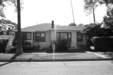 |
 |
 |
 |
 Mountain |
 Coast |
 InsideCity |
 Coast |
| InsideCity | 0.530 |  |
 |
 |
 |
 Store |
 Street |
 Kitchen |
 TallBuilding |
| TallBuilding | 0.720 |  |
 |
 |
 |
InsideCity |
 OpenCountry |
 Industrial |
| Street | 0.740 |  |
 |
 |
 |
 Bedroom |
 InsideCity |
 Mountain |
 Store |
| Highway | 0.840 |  |
 |
 |
 |
 OpenCountry |
 Industrial |
 Store |
 Forest |
| OpenCountry | 0.460 |  |
 |
 |
 |
 Coast |
 Street |
 Coast |
 Coast |
| Coast | 0.770 |  |
 |
 |
 |
 OpenCountry |
 OpenCountry |
 Highway |
 OpenCountry |
| Mountain | 0.820 |  |
 |
 |
 |
 Coast |
 Forest |
 OpenCountry |
 Bedroom |
| Forest | 0.910 |  |
 |
 |
 |
 Mountain |
 Mountain |
 Mountain |
| Category name | Accuracy | Sample training images | Sample true positives | False positives with true label | False negatives with wrong predicted label | ||||