Project 4 / Scene Recognition with Bag of Words
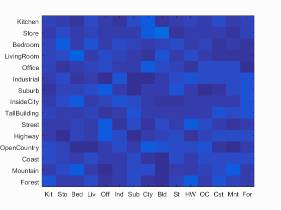
Fig. 1 Accuracy (mean of diagonal of confusion matrix) is 6.8%
The objective of this project is to perform image recognition. The procedure of solving this problem includes two steps. One is to develop image descriptors and second is to develop image classifiers. Two kinds of image descriptors are implemented, including tiny images and bag of sift descriptor. Also two kinds of classifiers are implemented, including nearest neighbor and support vector machine. I will also show how the spatial pyramid can further improve the recognition accuracy and the influence of vocabulary size. To compare our implementation results with chance performance, Fig. 1 shows the confusion matrix for chance performance.
Implementation and Results
1. Tiny Image Representation and Nearest Neighbor Classfier
The tiny image feature is one of the simplest image representations. In this section, I resized each image to 16x16 by scaling its dimensions down to make the smaller dimension equal to 16 and then cropping the other dimension.
The nearest neighbor classifier assigns each test feature into a particular category by finding the "nearest" training feature and assigning the test feature into the category of that training feature.
The accuracy of this implementation is 19.7% as shown in Fig. 2.
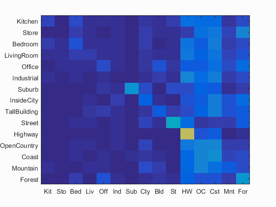
Fig. 2 Accuracy (mean of diagonal of confusion matrix) is 19.7%
2. Bag of SIFT Representation and Nearest Neighbor Classifier
In this section, I used bag of SIFT as the feature descriptor and still used nearest neighbor classifier. This technique has two steps, including building vocabulary based on SIFT features and getting bags of SIFT features. The function vl_dsift from VL feat is used to find dense SIFT features.
In the first step, the step size for vl_dsift is 5. More features will be obtained if the step size is smaller. A larger step size can be used in this step. After obtaining all SIFT features from all training images, one hundred thousand features are randomly sampled. Then I built the vocabulary with the size of 200 by using k-mean clustering method and vl-kmeans function from VL feat.
In the second step, the step size for vl_dsift is still 5. Each training and testing image is represented by a histogram of the developed vocabulary. In each image, each SIFT feature is assigned to the "nearest" bin of the vocabulary and the final histogram for each image is normalized.
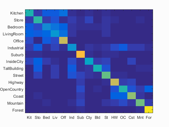
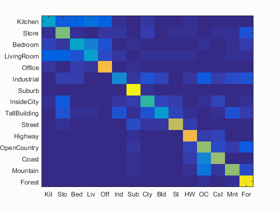
By implementing nearest neighbor classifier, the accuracy is 54.3%, as shown in Fig. 3(a), which is a big improvement from tiny image representation. When the step size in the second step is changed to 15, the computation time is about 100s and the accuracy is 46.9%, as shown in Fig. 3(b).
|
(a) Fig. 3 (a) Accuracy (mean of diagonal of confusion matrix) is 54.3%; (b) Accuracy (mean of diagonal of confusion matrix) is 46.9%. |
 (b)
(b)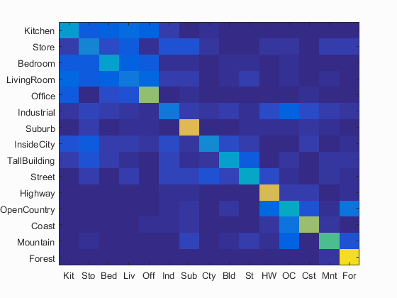
3. Bag of SIFT Representation and Linear SVM Classifier
In this section, we changed nearest neighbor classifier to linear support vector machine (SVM) classifier. 1-vs-all SVM is used, so totally 15 linear classifiers are trained by using training data. During training each classifier, vl_svmtrain from VL feat was used with lambda = 0.0001.
Then, each test descriptor was evaluated by all the trained classifiers. The most confident classifier with the largest residual won and the corresponding category was assigned.
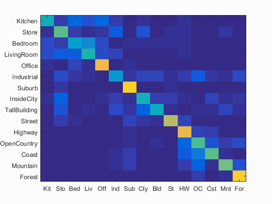
By implementing this algorithm, the accuracy is further improved 68.7%, as shown in Fig. 4(a). When the step size in deriving bags of SIFT features is changed to 15, the computation time is about 100s and the accuracy is 57.5%, as shown in Fig. 4(b).
|
(a) Fig. 3 (a) Accuracy (mean of diagonal of confusion matrix) is 68.7%; (b) Accuracy (mean of diagonal of confusion matrix) is 57.5%. |
 (b)
(b)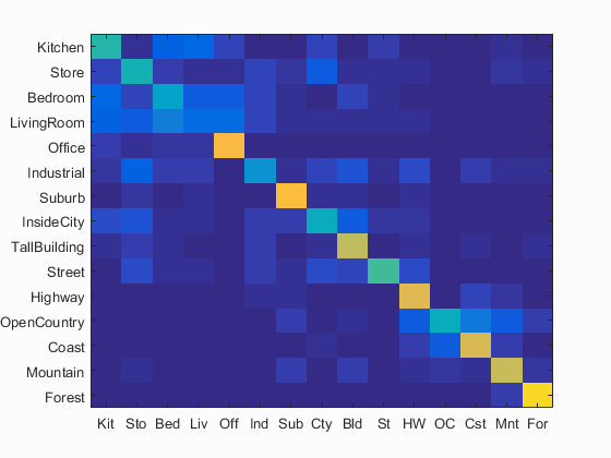
Extra
1. Spatial Pyramid
By adding spatial features, the image spatial information can be preserved with bag of SIFT representation and the recognition performance can be improved. I tested two classifiers, including nearest neighbor and linear SVM, and kept all parameters same. By adding one layer (4 bins) and forming 2-layer pyramid (5 bins), the accuracy for the nearest neighbor classifier and SVM is improved to 58% and 71.2 (Figs. 5(a) and 5(b)), respectively. By adding two layers (20 bins) and forming 3-layer pyramid (21 bins), the accuracy for the nearest neighbor classifier and SVM is improved to 59.7% and 74.1 (Figs. 5(c) and 5(d)), respectively.
|
(a) (c) Fig. 5 (a) Accuracy (mean of diagonal of confusion matrix) is 58.0%; (b) Accuracy (mean of diagonal of confusion matrix) is 71.2%; (c) Accuracy (mean of diagonal of confusion matrix) is 59.7%; (d) Accuracy (mean of diagonal of confusion matrix) is 74.1%. |
 (b)
(b)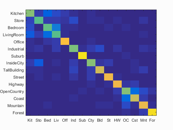
 (d)
(d)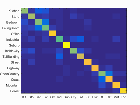
2. Vocabulary Size
Different vocabulary sizes were tried, including 10, 20, 50, 100, 200, 500, 1000, and 10000. I experimented this by using the combination of bag of SIFT and SVM. The spatial pyramid has only 1 layer. The variation of accuracy in the first seven cases of vocabulary size is shown in Fig. 6. The confusion matrix and performance for each scene when vocabulary size is 1000 are shown in Figs. 7 and 8, respectively. It is found that computation time increases with larger vocabulary size. Although the accuracy improves with larger vocabulary sizes, there is an improvement limitation. From Fig. 6, size of 200 is a good choice because of relatively high accuracy and short computation time.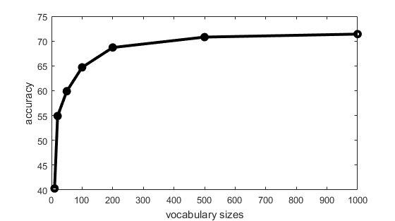
Fig. 6 Accuracy under different vocabulary sizes.

Fig. 7 Accuracy (mean of diagonal of confusion matrix) is 71.4%.
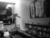
| Category name | Accuracy | Sample training images | Sample true positives | False positives with true label | False negatives with wrong predicted label | ||||
|---|---|---|---|---|---|---|---|---|---|
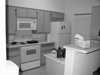
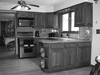
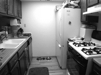
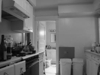
| Kitchen | 0.650 |  |
 |
 |
 |
 LivingRoom |
 LivingRoom |
 Bedroom |
 Bedroom |
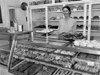
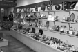
| Store | 0.670 | 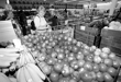 |
 |
 |
 |
 LivingRoom |
 Industrial |
 InsideCity |
 InsideCity |
| Bedroom | 0.420 | 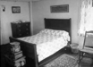 |
 |
 |
 |
 LivingRoom |
 InsideCity |
 TallBuilding |
 Office |
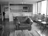
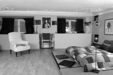
| LivingRoom | 0.440 |  |
 |
 |
 |
 Bedroom |
 Bedroom |
Store |
 Office |
| Office | 0.950 |  |
 |
 |
 |
 Kitchen |
Industrial |
 Bedroom |
 Kitchen |
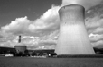
| Industrial | 0.590 | 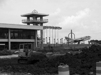 |
 |
 |
 |
 Street |
 Store |
TallBuilding |
 TallBuilding |
| Suburb | 0.960 |  |
 |
 |
 |
 Mountain |
 InsideCity |
 InsideCity |
 InsideCity |
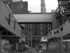
| InsideCity | 0.580 |  |
 |
 |
 |
 Industrial |
 Street |
 Highway |
 Street |
| TallBuilding | 0.830 |  |
 |
 |
 |
 Industrial |
 InsideCity |
 Coast |
 Street |
| Street | 0.710 |  |
 |
 |
 |
 InsideCity |
 Industrial |
 Highway |
 InsideCity |
| Highway | 0.840 |  |
 |
 |
 |
 Coast |
 Street |
 OpenCountry |
 OpenCountry |
| OpenCountry | 0.480 |  |
 |
 |
 |
 Mountain |
Highway |
 Coast |
 Coast |
| Coast | 0.840 |  |
 |
 |
 |
 Forest |
 Industrial |
 Highway |
 Highway |
| Mountain | 0.800 |  |
 |
 |
 |
 Forest |
 Forest |
Suburb |
 Coast |
| Forest | 0.950 |  |
 |
 |
 |
 OpenCountry |
 Mountain |
 Store |
| Category name | Accuracy | Sample training images | Sample true positives | False positives with true label | False negatives with wrong predicted label | ||||
Fig. 8 Performance for different scenes in 15 categories.