Project 4 / Scene Recognition with Bag of Words
This project's purpose was to classify images into categories based on their location. This writeup will explain the algorithms behind the cassification and the results obtained for certain configurations. I used two types of image representations and two types of classifiers during this project.
Table of Contents
- Background Information
- Algorithm: Tiny Image Representation
- Algorithm: Building a vocabulary
- Algorithm: Bag of SIFTs Representation
- Algorithm: Nearest Neighbor Classifier
- Algorithm: 1 vs. all SVM Classifier
- Results: Tiny Tmages and Nearest Neighbor
- Results: Bag of SIFTs and Nearest Neighbor
- Results: Bag of SIFTs + SVM
Background Information
For this project, I'm using a total of 3000 images: 1500 as my training set and 1500 as my testing set. Every image is in greyscale.
I am categorizing eahc of the image into one of the following 15 categories:
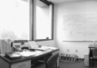
- Office
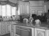
- Kitchen
- Lving Room
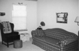
- Bedroom
- Store
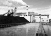
- Industrial
- Tall Building
- Incide City
- Street
- Highway
- Coast
- Open Country
- Mountain
- Forest
- Suburb
To classify the images, I first create image representations for each image. Afterwards, I use a supervised learning algorithm to classify my images into one of the 15 categories.
Algorithm: Tiny Image Representation
The tiny image representation is simply a 16x16 scaled down version of the original image. To create this representation, I simply resized each image to be 16x16, stored the 16x16 image as a length 256 vector, and normalized the vector to have 0 mean and an average magnitude of 1.
Algorithm: Building a vocabulary
Before being able to create the Bag of SIFTs Image Representation, a visual vocabulary must be learned. This visual vocabulary will be our "bags" in the bag of SIFTs. The following steps ouline how I implemented the creation of the visual vocabulary.
| Find SIFT features for each image | This was done using vlfeat's vl_dsift() function. The function takes in a step size which determines how many features are extracted from each image. It returns a size 128xN vector of features. |
| Store the features a matrix. | Since it is not known how many features are extracted from each image beforehand, I implmented a dynamically sized matrix. The matrix is initialized to size 128x1000 and will double in capacity whenever it runs out of columns to store features. Once all the features are inside the array, the excess columns will be removed. |
| Create the vocabulary with K means | Now that we have a matrix containing all of our features for each image, we can create our vocabulary with the K-Means algorithm. VL_Feat provides an inplementation with the function vl_kmeans(). The centers generated from Kmeans will be my vocabulary. |
Algorithm: Bag of SIFTs Representation
Now that we have our vocabulary, we can create out image representations for each image. The bag of SIFTs Representation is a normalized histogram of the closest vocabulary to each SIFT feature. The steps taken to implement this are outlined below.
| Find SIFT features for each image | This was also done using vlfeat's vl_dsift() function. It's important to note that the step sized used is less than the step size used when creating the vocabulary. It returns a size 128xN vector of features. |
| Assign each feature to a bag | Now, all of features obtained must be assigned to a bag. The vl_alldist2() function that VLFeat provides is used to compute the distance to each of the centers in the vocabulary. Once the distances are computed, each bag is assigned to the center with the minimum distance |
| Create the histogram | The representaiton each image will be a vector counting how many features fall into each of the vocabulary centers. MATLAB provides a function histcounts() used to create the histogram of features in bags. The image representation is then normalized so that the size of each image doesn't affect the result. This normalized histogram will be the final image representation. |
Algorithm: Nearest Neighbor Classifier
The nearest neighbor classifier simply assigns each testing image the same label of its nearest neighbor's label. The distance from each test image representation to all of the training image representations is calculated with VLFeat's vl_alldist2() funtion. The label of the training image with the minimum distance is assigned to the testing image.
Algorithm: 1 vs. all SVM Classifier
The 1 vs. All SVM classifier creates a hyperplane in each dimensions to compute confidences for each image to each label.
| Create the hyperplane with SVM for each category | This was also done using vlfeat's vl_svmtrain() function shown to the right. This function takes in training images, along with a label of -1 or 1. This is done in a loop that loops through each catecory. The label of an image is 1 when it's category matches the category of the loop's iteration and -1 otherwise. |
|
| Compute scores | Now that a hyperplane in each category is created with SVM, we can generate confidences for each training image. The code used to generate the score for a particular image j is shown to the right. |
|
| Assign labels to each image | Each image is assigned the label of category with the maximum score. |
Results: Tiny Tmages and Nearest Neighbor
This is the classification using the tiny image representation and the nearest neighbor classifier. Without normalizing the tiny images, I was getting 19.1% accuracy. After normalizing, I was getting 21.3% accuracy. The visualization is shown here:
Normalized Scene classification results visualization
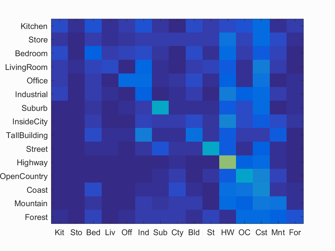 Accuracy (mean of diagonal of confusion matrix) is 0.213
Results: Bag of SIFTs and Nearest Neighbor
This is the classification using the Bag of SIFTS and Neariest Neighbor. There are several free variables: vocab_size, step size when generating vocab, and step size when creating histogram.
When generating the vocab, I kept the default vocab size of 200. I tried several step sizes including 15, 30, and 50. It appeared that the smaller the step size, the higher the accuracy, so I used the step size of 15.
For my implementation of the bag of wirds, I found that a step size of 5 when creating the histogram was giving me a good accuracy of 51.4% Due to run-time contraints, I set the step-size to 10 and obtained a 48.7% accuracy instead.
Fast Scene classification results visualization
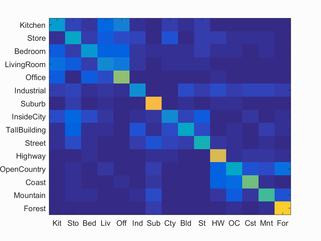 Accuracy (mean of diagonal of confusion matrix) is 0.487
Results: Bag of SIFTs + SVM
This was the most successful of the combinations I attempted.
Keeping the bag of sift's step size as 10, I attempted a variety of different lambdas: .00001, .0001, .001, .01, .1, 1, 10. The results are below. The highest accuracy was with the lambda of .001
| Lamda | .00001 | .0001 | .001 | .01 | .1 | 1 | 10 |
| Accuracy | .569 | .599 | .568 | .479 | .439 | .377 | .442 |
I was able to get an accuracy of 65% with the Bag of SIFTS step size as 5 instead of 10, however that doubles the run time from approx. 5 minutes to approx. 10 minutes. The results are below.
Accurate Scene classification results visualization
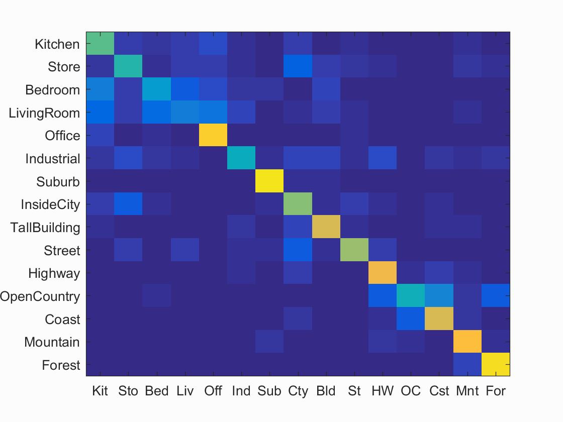
Accuracy (mean of diagonal of confusion matrix) is 0.641
| Category name | Accuracy | Sample training images | Sample true positives | False positives with true label | False negatives with wrong predicted label | ||||
|---|---|---|---|---|---|---|---|---|---|
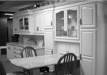
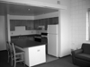
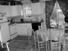
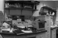
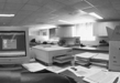
| Kitchen | 0.560 |  |
 |
 |
 |
 Bedroom |
 Bedroom |
 Store |
 Store |
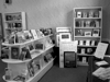
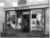
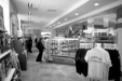
| Store | 0.470 |  |
 |
 |
 |
 Street |
 Street |
 Kitchen |
 InsideCity |
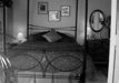
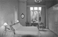
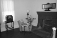
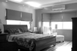
| Bedroom | 0.340 | 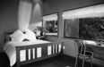 |
 |
 |
 |
 Kitchen |
 LivingRoom |
 LivingRoom |
 Store |
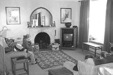
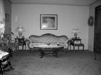
| LivingRoom | 0.220 |  |
 |
 |
 |
 Store |
 Street |
 Street |
 Kitchen |
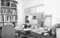
| Office | 0.880 | 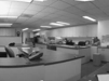 |
 |
 |
 |
 Bedroom |
 InsideCity |
 Kitchen |
 Bedroom |
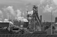
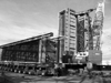
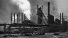
| Industrial | 0.410 | 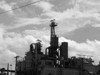 |
 |
 |
 |
 LivingRoom |
 Bedroom |
 Store |
 Store |
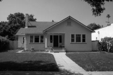
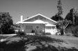
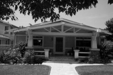
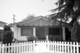
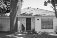
| Suburb | 0.940 | 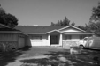 |
 |
 |
 |
 Store |
 Office |
 Store |
 InsideCity |
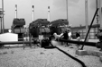
| InsideCity | 0.620 |  |
 |
 |
 |
 Store |
 Kitchen |
 Coast |
| TallBuilding | 0.760 |  |
 |
 |
 |
 Suburb |
 LivingRoom |
 InsideCity |
 Coast |
| Street | 0.650 |  |
 |
 |
 |
 Office |
 TallBuilding |
LivingRoom |
 Suburb |
| Highway | 0.800 |  |
 |
 |
 |
 InsideCity |
 Industrial |
 Industrial |
 OpenCountry |
| OpenCountry | 0.430 |  |
 |
 |
 |
 Coast |
 Highway |
 Coast |
 Coast |
| Coast | 0.760 |  |
 |
 |
 |
 OpenCountry |
 OpenCountry |
 OpenCountry |
 OpenCountry |
| Mountain | 0.840 |  |
 |
 |
 |
 Forest |
 Kitchen |
 Suburb |
 Coast |
| Forest | 0.930 |  |
 |
 |
 |
 Store |
 TallBuilding |
 Mountain |
 Mountain |
| Category name | Accuracy | Sample training images | Sample true positives | False positives with true label | False negatives with wrong predicted label | ||||