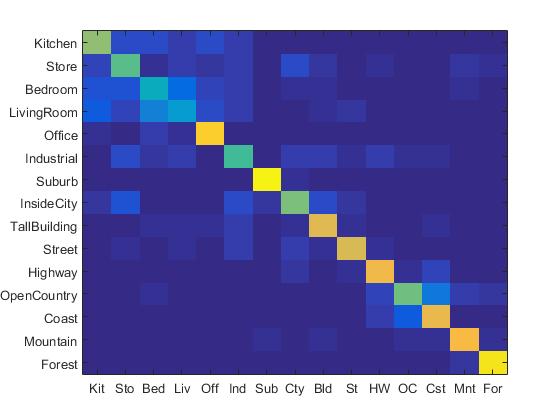
Example of a Confusion Matrix.

Code, Algorithms and Results

Part 1: Tiny images representation and nearest neighbor classifier

For tiny image feature, the images are resized into 16 by 16 resolution. In addition, the tiny images are also made to have zero mean and unit length. For nearest neighbor classifier, in order to classify a test feature into a category, the nearest training example is found, and the label of the nearest training example is assigned to the test case.

Some code for get_tiny_images.m is shown below:

for x=1:size_impath
  img=double(imresize(imread(image_paths{x}),[16,16]));% resize the image to 16*16 small image
  img=bsxfun(@minus,img,mean(img));%zero-mean and unit length
  image_feats(x,:)=reshape(img,[1,16*16]);
end

Some code for nearest_neighbor_classify.m is shown below:

size_image_feat=size(test_image_feats,1);
distance=vl_alldist2(train_image_feats',test_image_feats');
[~,min_index]=min(distance);
predicted_categories=cell(size_image_feat,1);
for i=1:size_image_feat
    predicted_categories{i}=train_labels{min_index(i)};
end

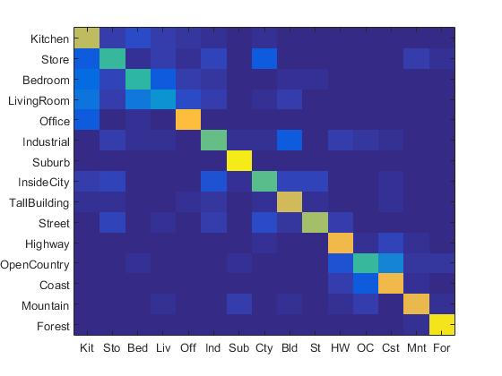
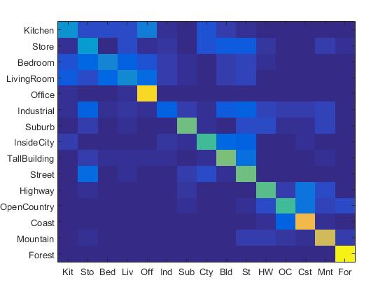
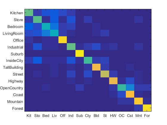
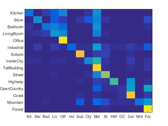
The confusion matrix of tiny images representation and nearest neighbor classifier is shown below:

Confusion Matrix of Tiny Image paired with Nearest Neighbor Classifier.

The accracy of tiny images representation and nearest neighbor classifier is 19.1%. It can be observed here that the accuracy of tiny images representation and nearest neighbor classifier is relatively low since this method neglects image contents which have high frequency. In addition, this method is not quite invariant to spatial or brightness shifts.

Part 2: Bag of SIFT representation and nearest neighbor classifier

In this part, a more sophisticated image representation, bags of quantized SIFT features, is implemented. First of all, a vocabulary of visual words is established. This vocabulary is formed by sampling many local features from training set and then clustering them with K-means. After the vocabulary of visual words is established, the SIFT representation needs to be built. In this part, the "step_size" parameter in build_vocabulary is set to be 30, and the "step_size" parameter in get_bags_of_sifts is set to be 5 to maximize accuracy and meanwhile reduce running time.

Some code for build_vocabulary.m is shown below:

for i = 1: size_image_path
    image = imread(image_paths{i});
    [~, SIFT_features] = vl_dsift(single(image),'fast','step',30);
SIFT_tot = [SIFT_tot,SIFT_features];
end

[centers, ~] = vl_kmeans(single(SIFT_tot), vocab_size);
vocab = centers';

Some code for get_bags_of_sifts.m is shown below:

for i = 1: image_path_size
    image = imread(image_paths{i});
    [~, SIFT_features] = vl_dsift(single(image),'fast','step',10);
    M = size(SIFT_features,2);
    D = vl_alldist2(single(SIFT_features),single(vocab'));
    
    for j = 1:M
        [~,I] = min(D(j,:));
        image_feats(i,I) = image_feats(i,I) + 1;
    end
    
    image_feats(i,:) = image_feats(i,:)/norm(image_feats(i,:));
end

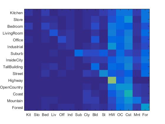
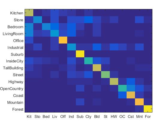
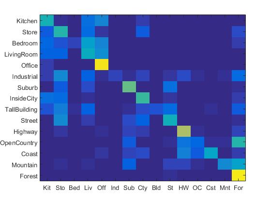
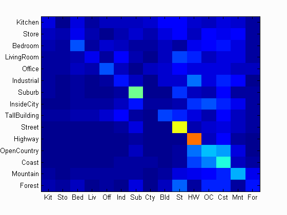
The confusion matrix of Bag of SIFT representation and nearest neighbor classifier is shown below:

Confusion Matrix of Bag of SIFT representation and nearest neighbor classifier.

When the step size is set to be 5, the accracy of Bag of SIFT representation and nearest neighbor classifier is 53.9%. However, the running time is 12 minutes. When the step size is set to be 10, the accuracy is 50%, and the running time is almost 5 minutes.

Part 3: Bag of SIFT representation and linear SVM classifier

Some code for svm_classify is shown below:

for i=1:length(training_cat)
    matching_indices=strcmp(training_cat{i},train_labels);
    [W(:,i), B(1,i)] = vl_svmtrain(train_image_feats', double(matching_indices*2-1), LAMBDA);
end

 for i=1:size_image_feat
       for j=1: length(training_cat)
           score(1,j)=test_image_feats(i,:)*W(:,j)+B(1,j);
       end 
       [~,index]=max(score);
       predicted_categories{i}=training_cat{index};
 end

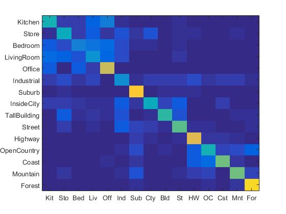
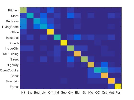
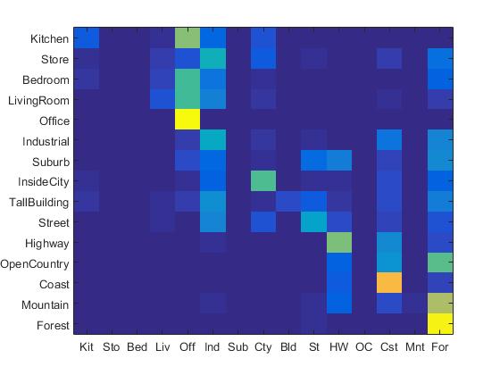
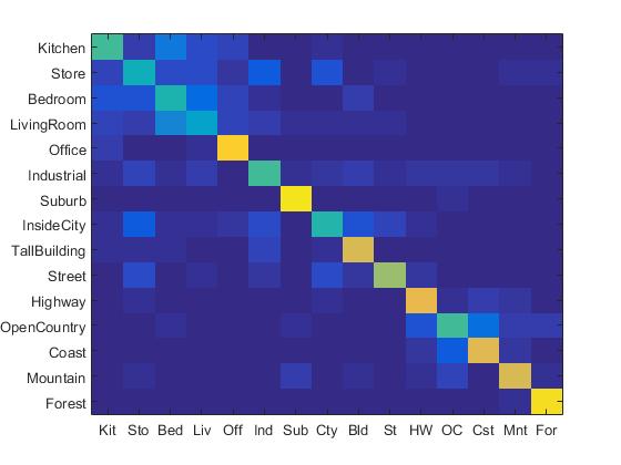
The confusion matrix of Bag of SIFT representation and linear SVM classifier is shown below:

Confusion Matrix of Bag of SIFT representation and linear SVM classifier.

In this part, the lambda value is set to be 0.0001. When the step size in bags of sifts is 5, the accracy of Bag of SIFT representation and linear SVM classifier is 67.5%. In order to reduce running time, the step size is set to be 10, the accuracy is 62.7%.

Some Extra Works

In this part, several extra point works are implemented. They include:

1. Experiment with many different vocabulary sizes and report performance
2. Experiment with lambda value in SVM and report performance
3. NBNN (Naive Bayes Nearest Neighbor) Classifier

Experiment with many different vocabulary sizes and report performance

Experiment with many different vocabulary sizes and report performance

For this part, different vocabulary sizes include: 10, 20, 50, 100, 200, 400, 1000, 10000 are tested under bags of SIFT features and nearest neighbor pipeline. The highest accuracy is achieved when the vocabulary size is 1000. The highest accuracy is 55%. The figure below shows the accuracy and vocab_size.

Experiment with many different vocabulary sizes

It can be observed here that when the accuracy increases with the increase of vocabulary size. However, when vocabulary reaches 200 and above, the accuracy tend to increase for a very limited amount. Moreover, it also take much longer to run the program when the vocabulary size reaches above 500. So setting vocabulary size to 200 is a reasonable choice.

Experiment with lambda value in SVM and report performance

Experiment with lambda value in SVM and report performance

For this part, different lambda value in SVM include: 10, 1, 0.1, 0.01, 0.001, 0.0001, 0.00001 are tested under bags of SIFT features and svm classifier pipeline. The highest accuracy is achieved when the lambda value is 0.0001. The highest accuracy is 67.9%. The figure below shows the accuracy and lambda value.

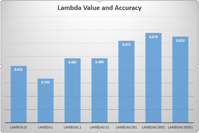
Experiment with lambda value in SVM

Implementation of NBNN (Naive Bayes Nearest Neighbor) Classifier

In this part, NBNN (Naive Bayes Nearest Neighbor) classifier is implemented. This is a trivial NN-based classifier which calculates NN-distances in the space from image descriptors. It computes direct distances without descriptor quantization. The advantage of NBNN is simple, effective and no learning/training process is required.

The algorithm of NBNN is shown below:

algorithm of NBNN

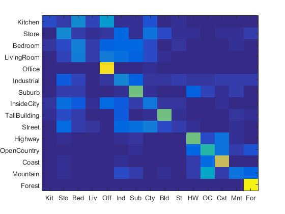
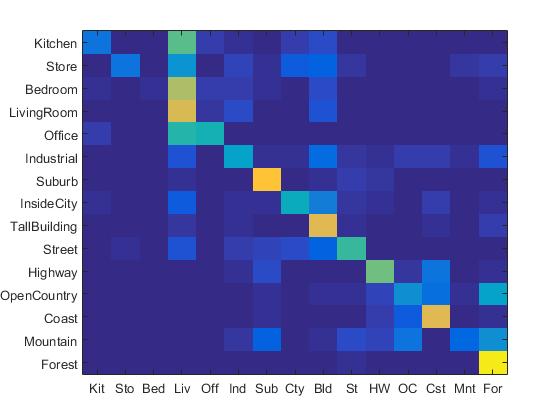
It has been illustrated in some literature that the performance of NBNN ranks among the top leading learning-based image classifiers. However, in this project, NBNN takes extremely long time to run since it compares every features. It is very time-consuming to run NBNN in this project even if the step-size is set to be quite large. In order to reduce the running time, the step-size is set to be 30, and the accuracy is 15.1%. The confusion matrix by implementing NBNN classifier is shown below:

Confusion Matrix of the Implementation of NBNN

Highest Accuracy Result

The highest accuracy is achieved when I set the vocab size to be 1000, step size in build vocabulary to be 10, step size in get bags of sift to be 3, and lambda in svm to be 0.0001. The highest accuracy is 74.2%.

Scene classification results visualization

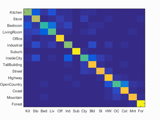
Accuracy (mean of diagonal of confusion matrix) is 0.742

Category name	Accuracy	Sample training images		Sample true positives		False positives with true label		False negatives with wrong predicted label
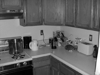
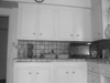
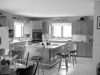
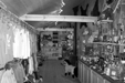
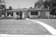
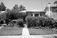
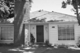
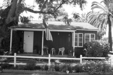
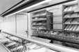
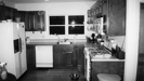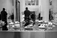
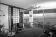
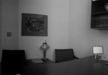
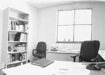
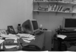
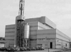
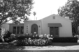
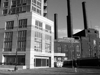
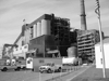
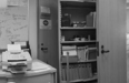
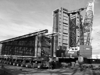
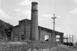
Kitchen	0.640					Office	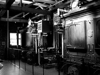Industrial	Industrial	Industrial
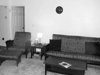
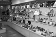
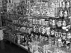
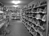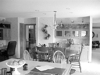
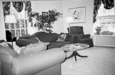
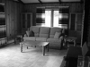
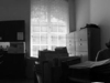
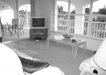
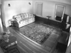
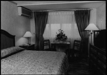
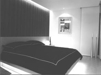
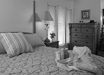
Store	0.700					LivingRoom	LivingRoom	Office	Bedroom
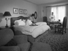
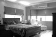
Bedroom	0.490					LivingRoom	Kitchen	Store	LivingRoom
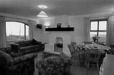
LivingRoom	0.550		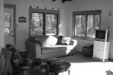			Industrial	Bedroom	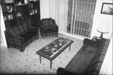Bedroom	Kitchen
Office	0.920		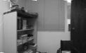			Bedroom	InsideCity	Bedroom	Kitchen
Industrial	0.620		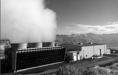			Bedroom	InsideCity	OpenCountry	Bedroom
Suburb	0.960		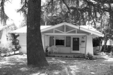			Industrial	OpenCountry	InsideCity	Store
InsideCity	0.540					Store	TallBuilding	TallBuilding	TallBuilding
TallBuilding	0.850					Industrial	Street	InsideCity	Coast
Street	0.800					LivingRoom	Store	Forest	Highway
Highway	0.860					OpenCountry	Store	Forest	Store
OpenCountry	0.540					Mountain	Highway	Coast	Coast
Coast	0.850					OpenCountry	TallBuilding	OpenCountry	Highway
Mountain	0.840					LivingRoom	OpenCountry	Coast	Coast
Forest	0.970					Store	Street	Mountain	Mountain
Category name	Accuracy	Sample training images		Sample true positives		False positives with true label		False negatives with wrong predicted label