Project 4 / Scene Recognition with Bag of Words
Example of a right floating element.
Project is about image recognition. It is divided into two devisions. First is the feature extraction part and second is the classification part. In Extraction- we use Tiny images and Bag of SIFT features, Here experiment is done with GIST feature and without it. Multiple scales are tried. Furthermore, spatial pyramid method is tried to check the increase in the accuracy.Experiment with many different vocabulary sizes was made.
- Tiny images
- Bag of SIFT features
- Nearest neighbour
- SVM
- Gist descriptor
- Spatial pyramid
- Soft asignment
- Experiment with features at multiple scales
- Experiment with many different vocabulary sizes and report performance
- Tiny Images
- Bag of SIFT features
- Nearest neighbour algorithm This is one of the classification algorithms. Nearest algorithm checks the nearest value from the trained data and classifies itself to that class. The KNN algorithm considers K nearest trained data and classifies with the maximum occuring class in from the algorithm.
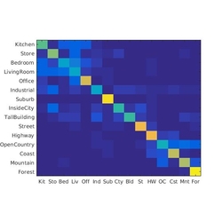
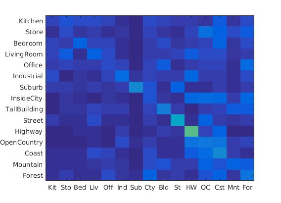
- Tiny images and NN Accuracy (mean of diagonal of confusion matrix) is 0.201
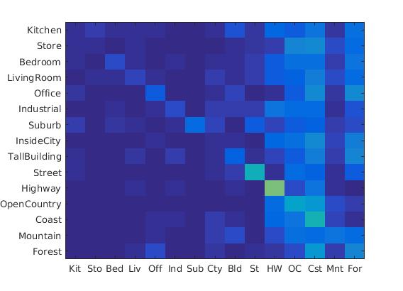
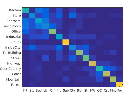
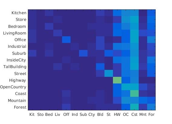
- Bag of words and NN Accuracy (mean of diagonal of confusion matrix) is 0.495
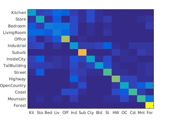
- Bag of words and NN and GIST Accuracy (mean of diagonal of confusion matrix) is 0.607
- SVM classifier
- Tiny images and SVM Accuracy (mean of diagonal of confusion matrix) is 0.193
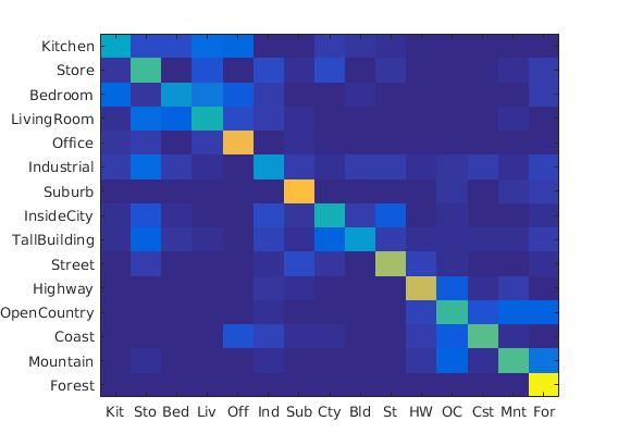
- Bag of words and SVM Accuracy (mean of diagonal of confusion matrix) is 0.539
- Spatial pyramid
- Soft Assignment
- Experiment with features at multiple scales
- 4*4 scale: 0.203
- 8*8 scale: 0.214
- 16*16 scale: 0.201
- 64*64 scale : 0.177
- 128*128 scale: 0.167
- Experiment with many different vocabulary sizes and report performance.
- size 10: 0.367
- size 20: 0.432
- size 50: 0.501
- size 100: 0.513
- size 200: 0.523
- size 400: 0.527
- size 1000: 0.531
- size 10000: 0.532
- GIST descriptors
The tiny image feature, inspired by the work of Torralba, Fergus, and Freeman. Image is resized to a small, fixed resolution.This is not a particularly good representation, because it discards all of the high frequency image content. It is invarient to brightness. Here it is resized to 16*16 size and described it as feature
%example code
for i = 1:1:length(image_paths)
    s=strjoin(image_paths(i));
    image=imread(s);
    image1=imresize(image,[16 16]);
    image_feats(i,:)=reshape(image1,[1,256]);
Here the SIFT features are extracted from the image and then using Kmeans agorithm, they are divided into clusters. This cluster acts as vocabulary for the bag of sift features algorithm.
Build Vocabulary
sift_feat=[];
for i = 1:1:length(image_paths)
    s=strjoin(image_paths(i));
    img=imread(s);
    [locations, SIFT_features] = vl_dsift(single(img) ,'fast',  'step' , 10) ;
    sift_feat=[SIFT_features'; sift_feat']';
    disp('for loop ')
    disp(i)
end
X=sift_feat;
K=vocab_size;
[centers, assignments] = vl_kmeans(single(X), K);
size(centers)
vocab=centers;
Then we can take the test image and extract SIFT features from it. Check which is the nearest cluster. We count the number of SIFT features for each cluster. This act as the features for classification algorithm.
Bag of SIFT
load('vocab.mat')

vocab_size = size(vocab, 2);

nearest_cluster=zeros(vocab_size,1);
for i = 1:1:length(image_paths)
    s=strjoin(image_paths(i));
    img=imread(s);
    [locations, SIFT_features] = vl_dsift(single(img) ,'fast', 'step' , 5) ;
    D = vl_alldist2(single(SIFT_features),single(vocab));
    [mini1,I]=min(D, [], 2);


   %Normal bag of words!!!

    for j=1:size(I,1)
        nearest_cluster(I(j,1),1)=nearest_cluster(I(j,1),1)+1;
    end

    nearest_cluster=normc(nearest_cluster);
    image_feats(i,:)=nearest_cluster(:,1)';
Nearest neighbour
D = vl_alldist2(train_image_feats',test_image_feats');
[mini1,I]=min(D, [], 2);
predicted_categories=train_labels(I);
RESULTS 1
|
SVM is a linear classifier. We have implemented 1-vs-all linear SVMS to operate in the bag of SIFT feature. Linear classifiers are one of the simplest possible learning models. The feature space is partitioned by a learned hyperplane. The test values are divided whether it is in this side of hyperplane or the another side. So it give the value(-ve in our case). We then choose the minimum value as the class for the data set.
%testfeat 1500*200
for j=1: size(test_image_feats,1)
    output=zeros(size(num_categories));
    output=double(output);
    for i=1:num_categories
        size(W(i,:));
        size(train_image_feats(j,:)');
        %disp('output:')
        output(i,1)= double(W(i,:))*double(test_image_feats(j,:))'+B(i);
    end
    %size(output);
    %disp('min of ans');
    [mini1,I]=max(output,[],1);
    %size(I)
    a(j,1)=categories(I);

end
predicted_categories=a;
RESULTS 1

|
Here we divide the image into 2 scales. First one is the complete image itself. Second one is the 4*4 grid. Of image. Thus to divide the image into 4 parts. For eac of the five images, we calculate the SIFT features seperately and then concatinate and send them to the classifier. The performance improves than the normal implementation.
%this is for 2nd scale of pyramid. Such is done for four other parts.
%...
%...
I2=img(size(img,1)/2+1:size(img,1),1:size(img,2)/2,:);

[locations, SIFT_features] = vl_dsift(single(I2) ,'fast', 'step' , 5) ;
D = vl_alldist2(single(SIFT_features),single(vocab));
[mini22,I22]=min(D, [], 2);
for j=1:size(I22,1)
   nearest_cluster2(I22(j,1),1)=nearest_cluster2(I22(j,1),1)+1;
end

nearest_cluster2=normc(nearest_cluster2);
image_feats2=nearest_cluster2(:,1)';
%...
%...
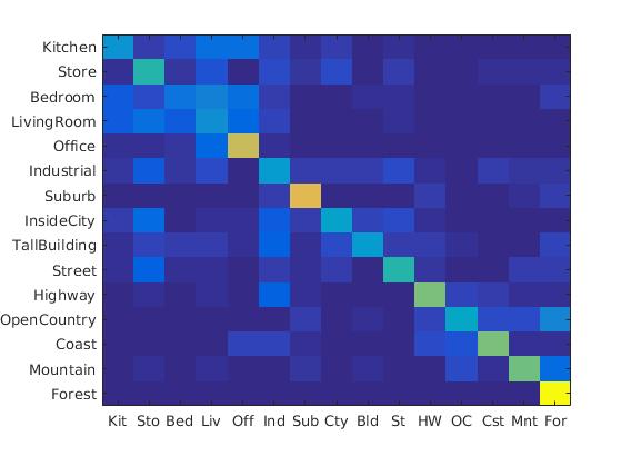
Spatial pyramid accuracy:
Accuracy increased from 0.495 to 0.560 after spatial Pyramid assignment
Here we put the weight of the sift feature instead of count while putting into cluster set. Thus instead of puting the count we put the weight of the cluster.The accuracy increases modestly with soft assignment.
%...
%...
s=strjoin(image_paths(i));
img=imread(s);
[locations, SIFT_features] = vl_dsift(single(img) ,'fast', 'step' , 5) ;
D = vl_alldist2(single(SIFT_features),single(vocab));
[mini1,I]=min(D, [], 2);
for j=1:size(I,1)
        nearest_cluster(I(j,1),1)=nearest_cluster(I(j,1),1)+mini1(j,1); % Here we used to add one for count.. here we are adding the weight
end
%...
%...
Soft assignment:
Accuracy increased from 0.495 to 0.532 after soft assignment
Following were the results with different scales:
Diagrams of 4*4 scale, 64*64 scale, 128*128 scale
|
Following were the results with different vocabulary size:
Here we have 16 bins. And 4 scales. And 8 orientations. Thus we get 512 dimention of features. Thus the SIFT are converted to 512 dimentional features.
features=nearest_cluster(:,1)';
param.imageSize = [256 256]; % it works also with non-square images
param.orientationsPerScale = [8 8 8 8];
param.numberBlocks = 4;
param.fc_prefilt = 4;
[gist1, param] = LMgist(img, '', param);
image_feats(i,:)=[features,gist1];
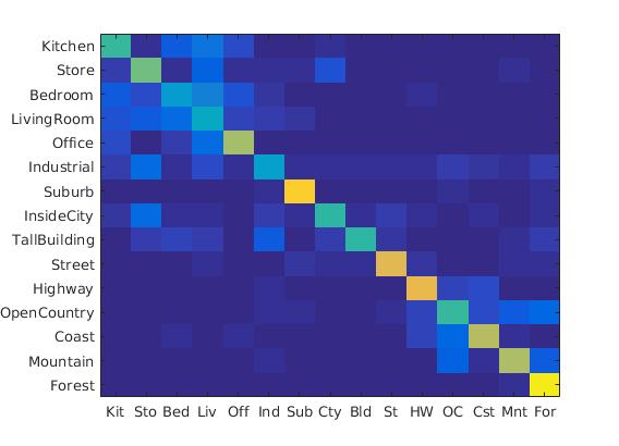
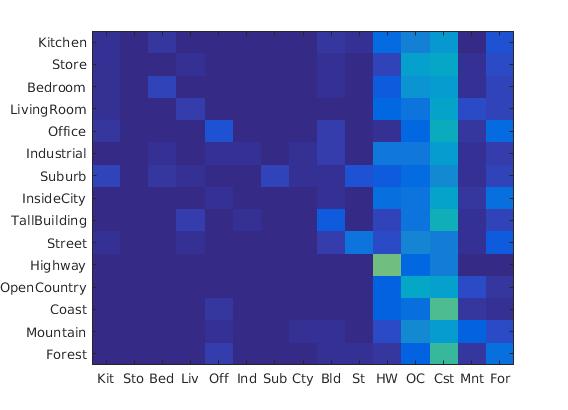
GIST accuracy:
Accuracy: 0.625

Accuracy (mean of diagonal of confusion matrix) is 0.625
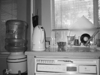
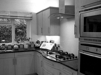
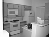
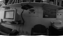
| Category name | Accuracy | Sample training images | Sample true positives | False positives with true label | False negatives with wrong predicted label | ||||
|---|---|---|---|---|---|---|---|---|---|
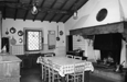
| Kitchen | 0.560 |  |
 |
 |
 |
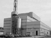
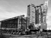
 Industrial |
 Forest |
 Highway |
 Forest |
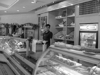
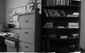
| Store | 0.610 | 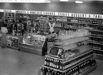 |
 |
 |
 |
 Office |
 TallBuilding |
 TallBuilding |
 Coast |
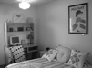
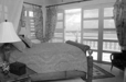
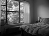
| Bedroom | 0.370 |  |
 |
 |
 |
 InsideCity |
 Store |
 OpenCountry |
 Mountain |
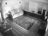
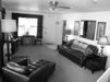
| LivingRoom | 0.390 |  |
 |
 |
 |
 Office |
 Kitchen |
 Bedroom |
 Office |
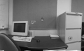
| Office | 0.750 | 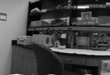 |
 |
 |
 |
 Mountain |
 Bedroom |
 Industrial |
 InsideCity |
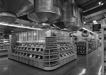
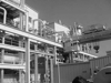
| Industrial | 0.380 | 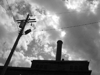 |
 |
 |
 |
 LivingRoom |
 TallBuilding |
 InsideCity |
 Store |
| Suburb | 0.930 | 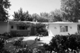 |
 |
 |
 |
 Coast |
 InsideCity |
 Kitchen |
 Street |
| InsideCity | 0.490 |  |
 |
 |
 |
 Suburb |
 Coast |
 TallBuilding |
 Store |
| TallBuilding | 0.500 |  |
 |
 |
 |
 Store |
 Forest |
 LivingRoom |
 Coast |
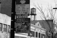
| Street | 0.810 |  |
 |
 |
 |
 Kitchen |
 Store |
 Highway |
 Suburb |
| Highway | 0.810 |  |
 |
 |
 |
 Suburb |
 Industrial |
 Coast |
 Mountain |
| OpenCountry | 0.430 |  |
 |
 |
 |
 Forest |
 Kitchen |
 Suburb |
 Coast |
| Coast | 0.710 |  |
 |
 |
 |
 Mountain |
 Mountain |
 InsideCity |
 OpenCountry |
| Mountain | 0.680 |  |
 |
 |
 |
 Store |
 Bedroom |
 Kitchen |
 Forest |
| Forest | 0.960 |  |
 |
 |
 |
 Mountain |
 Street |
 Suburb |
Kitchen |
| Category name | Accuracy | Sample training images | Sample true positives | False positives with true label | False negatives with wrong predicted label | ||||