Project 4: Scene Recognition with Bag of Words
Step 1: Normalization
I resize the image to 16*16 dimensions. All pixels are juxtapozed in a row and then zero-meaned.
Step 2: Vocabularies
100 random sift features are selected for each image. K-means with 400 cluster input is ran to make the vocabularies.
In order to build vocabulary, we need to get the sift feature of each image. However, an image could have over 100,000 interesting points where each of them has 128 dimensions. So what I did, based on the random permutation (Non-repeatable random number), I chose 100 samples out of all the provided interest points by sift feature command. Finally, we will obtain a matrix which holds all these 100 sample sift feature for all the images. So, if we have 1500 images, we will have 150000 sample points where each of then has 128 dimension. Then based on the provided vocabulary size, we define the number of clusters and implement k-means clustering to assign each sample to a cluster where the default number of clusters where 400. The code below provides a good explanation of what I coded for building vocabulary.
% running Kmeans
[centers, ~] = vl_kmeans(single(SIFTS_features), Size_of_Vocabulareis);
Step 3: Bag of Sift
Much larger sift features are used in this step to buld vocal histogram. Matlan knnsearch classifies the features to the 400 clusters. kd-tree is utilized here for computational speed gain. Also, I added the normalization.
load('vocab.mat')
vocab_size = size(vocab, 1);
image_feats = zeros(length(image_paths),vocab_size);
Mdl = KDTreeSearcher(vocab); % constructing the kd-tree here
for i = 1:length(image_paths)
    [~, SIFT_features] = vl_dsift(single(imread(image_paths{i})));
    sift_feature_rand = single(SIFT_features(:,randperm(size(SIFT_features,2),2000)));
    Idx = knnsearch(Mdl,sift_feature_rand'); % searching by using kd-tree
    [a,b] = hist(Idx,unique(Idx)); % a represents counting number in each cluster, and b will provide the index of the cluster
    image_feats(i,b) = a;
    feature = image_feats(i,:) - mean(image_feats(i,:)); % zero mean
    feature = feature./sqrt(sum(feature.^2)); % unit length
    image_feats(i,:) = feature;
end
Step 4: Gabor filter and Gist Features
WIKIPEDIA algorithm is used for gabor filtering
sigma_x = sigma;
sigma_y = sigma/gamma;
% Bounding box
nstds = 3;
xmax = max(abs(nstds*sigma_x*cos(theta)),abs(nstds*sigma_y*sin(theta)));
xmax = ceil(max(1,xmax));
ymax = max(abs(nstds*sigma_x*sin(theta)),abs(nstds*sigma_y*cos(theta)));
ymax = ceil(max(1,ymax));
xmin = -xmax; ymin = -ymax;
[x,y] = meshgrid(xmin:xmax,ymin:ymax);
% Rotation
x_theta=x*cos(theta)+y*sin(theta);
y_theta=-x*sin(theta)+y*cos(theta);
gb= exp(-.5*(x_theta.^2/sigma_x^2+y_theta.^2/sigma_y^2)).*cos(2*pi/lambda*x_theta+psi);
Step 5: Nearest Neighbor
For KNN K=1 lead to the best results in my case.
Step 6: SVM Classifier (RBF) kernel
MATLAB fitcsvm was leveraged for kernel SVM training since vl_svmtrain is only linear implementation.
step 7: Reporting the results
| Feature | Classifier | Accuracy |
| Random | Random | 7 |
| Pixels | KNN | 23 |
| Pixels | SVM - RBF | 20 |
| SIFT | KNN | 50 |
| SIFT | SVM - RBF | 71 |
Confusion matrix
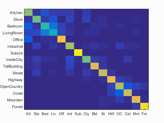
Accuracy = 0.710