Project 4 / Scene Recognition with Bag of Words

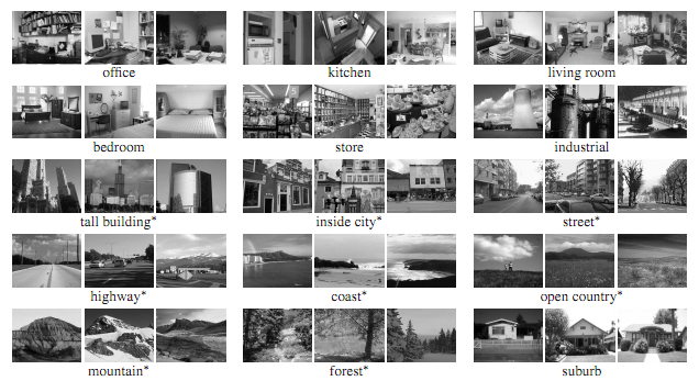
Example scenes from of each category in the 15 scene dataset. Figure from Lazebnik et al. 2006.

My scene recognition pipeline has two parts. I used the 15 scene dataset and implemented the following:

Part 1: Feature Extraction

1. Tiny image representation. Originally created by Torralba, Fergus, and Freeman. I simply resized each image to 16x16 and used the 256 pixels as a feature. I experimented with normalizing the features and making their mean 0.
2. SIFT Features
3. gist descripters. I used the gist decripters originally implemented by Aude Oliva, Antonio Torralba.

Part 2: Machine Learning

1. Nearest Neighbor
2. Linear Support Vector Machine

Experiments

1. Tiny Image with Nearest Neighbors

   Here, I ran tiny image with slight variations and then used nearest neighbors on those features. The variations are:
   • Just 256 pixels. The results were:
     

     
     Using tiny image representation for images
     Elapsed time is 12.498010 seconds.
     Using nearest neighbor classifier to predict test set categories
     Elapsed time is 1.961715 seconds.
     Accuracy = 0.191
     

     This was expected. You can see the full results here.
   
   
   • Just 256 pixels, but with normalization. I normalized the features to unit length. The results were:
     

     
     Using tiny image representation for images
     Elapsed time is 12.452074 seconds
     Using nearest neighbor classifier to predict test set categories
     Elapsed time is 1.543277 seconds.
     Accuracy = 0.199
     

     This was expected. I got a small boost in performance (0.199 vs 0.191).
     I did not expect it to take slightly less time, although I might be reading too much into it.
     You can see the full results here.
   
   
   • Just 256 pixels, but with normalization and zero mean. I normalized the features to unit length and set the mean to 0 by subtracting the old mean from each element in the feature. The results were:
     

     
     Using tiny image representation for images
     Elapsed time is 12.946300 seconds.
     Using nearest neighbor classifier to predict test set categories
     Elapsed time is 1.083529 seconds.
     Accuracy = 0.147
     

     This was very unexpected. I got a considerable loss in performance (0.147 vs 0.191) and it took longer to run.
     You can see the full results here.
     



2. Bag of SIFT with Nearest Neighbors

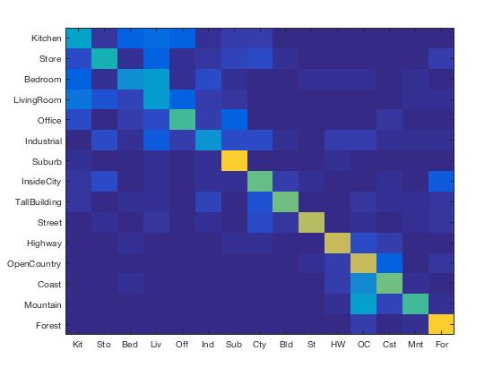
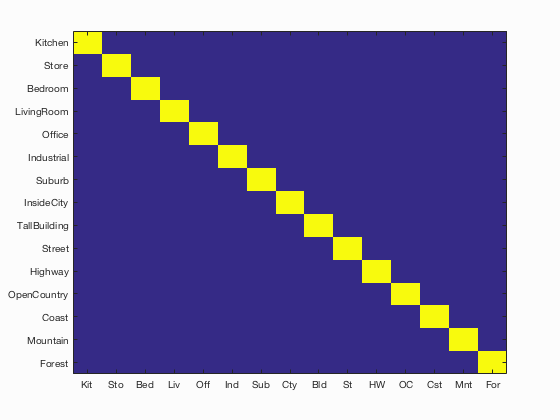
   I first ran SIFT with a vocab size of 200 and step size of 10. Results:

   
   Using bag of sift representation for images
   Elapsed time is 244.782265 seconds.
   Using nearest neighbor classifier to predict test set categories
   Elapsed time is 2.066009 seconds.
   Accuracy = 0.513
   

   Confusion matrix
   This was expected. As you can see, the creating a vocabulary and extracting SIFT features too about 4 minutes.
   I got an accuracy of 51%



3. Bag of SIFT with Linear SVMs

   Again, I used a vocab size of 200 and step size of 10. I varied Lambda to get the best performance.
   First I went through orders of magnitude, going from 0.1 to 10^-7. The results were:

   Lambda	10^-1	10^-2	10^-3	10^-4	10^-5	10^-6	10^-7
   Accuracy	0.4413	0.5387	0.5853	0.6313	0.5853	0.5507	0.5133
   Time (s)	0.8738	0.7585	0.9060	1.470	2.2398	6.6108	26.5470

   Plotting these:
   
   
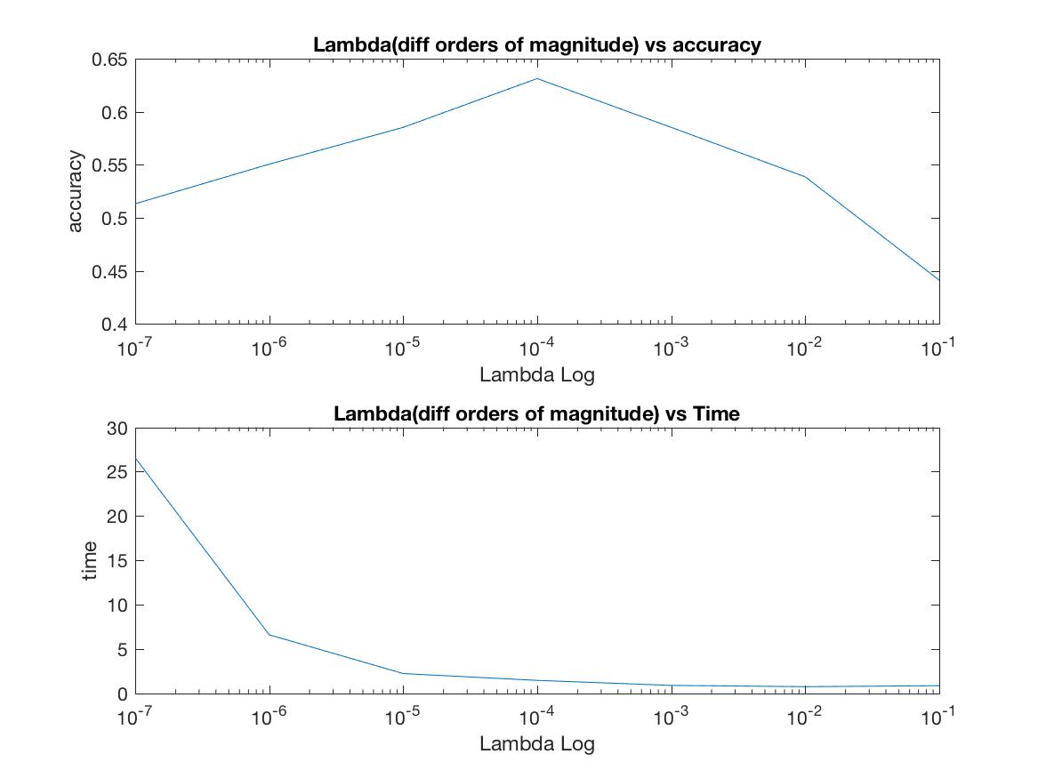   As you can see, there is a clear peak at 10^-4. So I started fine tuning.
   I ran it again but with Lambda varying from 0.0001 to 0.0009 in increments of 0.0001.

   Lambda	0.0001	0.0002	0.0003	0.0004	0.0005	0.0006	0.0007	0.0008	0.0009
   Accuracy	0.6287	0.6247	0.6180	0.6100	0.5987	0.5987	0.5967	0.6027	0.5953
   Time (s)	1.212	1.0172	0.8319	0.8044	0.8769	0.8388	0.8402	0.7931	1.0674

   Plotting these:
   
   Since 0.0001 performed the best, I used that value for future experiments.
   
   After this, I varied the vocab size. I experimented with parallel processing by using parpool to create a cluster locally and then using parfor loops. The result was

   Size	10	20	50	100	200	400	1000
   Accuracy	0.490	0.391	0.616	0.590	0.632	0.634	0.631

   
   
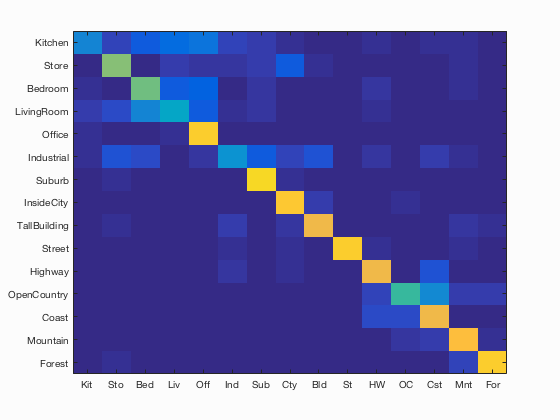
   Here is the confusion matrix for Lambda = 0.0002 and Vocab Size = 400: 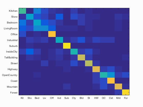The accuracy was 0.627 .You can see the full results here.

4. gist with Nearest Neighbors

   Using only gist features, I got a small increase in accuracy. Results:

   
   Using bag of gist representation for images
   Elapsed time is 308.598544 seconds.
   Using nearest neighbor classifier to predict test set categories
   Elapsed time is 4.023655 seconds.
   Accuracy (mean of diagonal of confusion matrix) is 0.561
   

   Confusion matrix
   Creating gist features took longer to extract than SIFT (5 minutes vs 4 minutes). There was a 3% increase in accuracy.



5. gist with Linear SVMs

   I varied Lambda to get the best performance.
   First I went through orders of magnitude, going from 0.1 to 10^-7. The results were:

   Lambda	10^-1	10^-2	10^-3	10^-4	10^-5	10^-6	10^-7
   Accuracy	0.2927	0.5720	0.6513	0.6913	0.6807	0.6493	0.6367
   Time (s)	0.9898	0.9484	1.0137	1.5346	4.9265	17.2567	23.6776

   Plotting these (Note the Y axis in the first plot is accuracy, and time in the second plot.):
   
   
   As you can see, there is a clear peak at 10^-4. So I started fine tuning.
   I ran it again but with Lambda varying from 0.0001 to 0.0009 in increments of 0.0001.

   Lambda	0.0001	0.0002	0.0003	0.0004	0.0005	0.0006	0.0007	0.0008	0.0009
   Accuracy	0.6967	0.6967	0.6847	0.6673	0.6573	0.6767	0.6633	0.6520	0.6687
   Time (s)	1.5756	1.268	1.1900	1.1118	1.1181	1.0523	1.1142	1.1592	1.201

   Plotting these (Note the Y axis in the first plot is accuracy, and time in the second plot.):
   
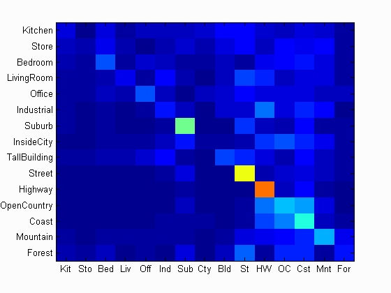
   Since 0.0001 and 0.0002 performed equally well and 0.0002 took less time, I used 0.0002 as my Lambda value for further experimetnts.
   Here is the confusion matrix for Lambda = 0.0002: The accuracy was 0.687 . This is the better than bag of SIFT by about 0.07. You can see the full results here.




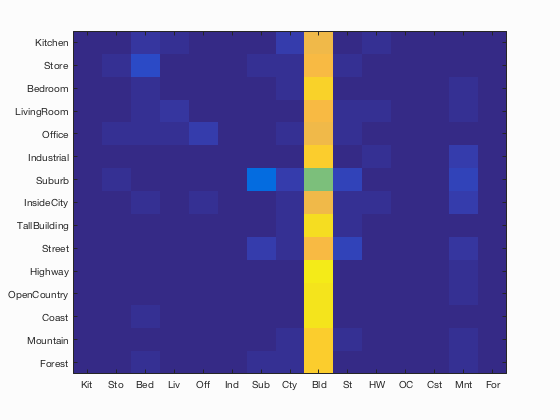
6. Combining features

   Thinking the more the merrier, I first combined all the three feature representations above and classified them using SVM.
   the results were dismal. I got only 9%. The confusion matrix is:
   
   I figured the tiny image representation might be skewing things on account of it's low information features. I combined gist and SIFT and the results were pretty good. I achieved around 77%. It achieved more than 90% accuracy for Suburb (95%), Street(91%) and Forest (92%)! The result was:

   Scene classification results visualization

   
   Accuracy (mean of diagonal of confusion matrix) is 0.768

   Category name	Accuracy	Sample training images		Sample true positives		False positives with true label		False negatives with wrong predicted label
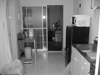
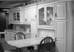
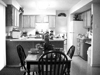
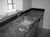
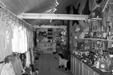
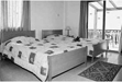
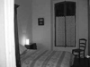
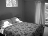
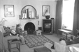
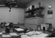
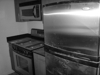
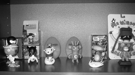
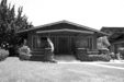
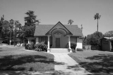
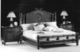
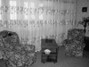
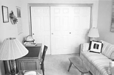
   Kitchen	0.650					Bedroom	Bedroom	Bedroom	Store
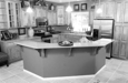
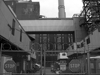
   Store	0.660					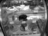Kitchen	Bedroom	TallBuilding	Kitchen
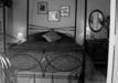
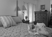
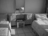
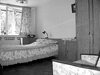
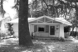
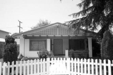
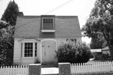
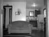
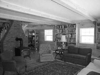
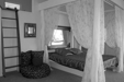
   Bedroom	0.570					LivingRoom	LivingRoom	OpenCountry	LivingRoom
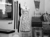
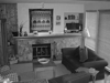
   LivingRoom	0.450					Bedroom	Bedroom	Bedroom	Bedroom
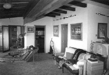
   Office	0.890					Kitchen	Bedroom	Kitchen	Kitchen
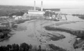
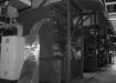
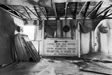
   Industrial	0.750					Store	Bedroom	Kitchen	Store
   Suburb	0.950					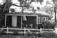LivingRoom	Bedroom	Kitchen	InsideCity
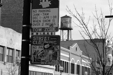
   InsideCity	0.790					Highway	Industrial	Kitchen	TallBuilding
   TallBuilding	0.880					InsideCity	LivingRoom	InsideCity	Store
   Street	0.910					Store	InsideCity	Mountain	InsideCity
   Highway	0.830					Coast	OpenCountry	Coast	Bedroom
   OpenCountry	0.590					Mountain	LivingRoom	Coast	Highway
   Coast	0.830					Industrial	OpenCountry	OpenCountry	Suburb
   Mountain	0.850					TallBuilding	Kitchen	Coast	Forest
   Forest	0.920					Mountain	OpenCountry	Store	TallBuilding
   Category name	Accuracy	Sample training images		Sample true positives		False positives with true label		False negatives with wrong predicted label

Weird result

I tried using Olivier Chapelle's SVM MATLAB code with an RBF kernel but it gave me 100% accuracy every time. Something was clearly wrong. Here is the confusion matrix I got:

Results

In the end, I managed to achieve about 76.8% accuracy by combining gist and SIFT features. I could have gotten better results by accounting for different spatial scales, using more optimized values for stepsize, image size etc. and using different SVM kernels. I will look into them in the future. I also couldn't finish performing cross validation which would have given me a more honest idea of the accuracy of my model. I tried running the code on GT PACE High Performance Cluster but couldn't get it working.

Data

You can see the confusion matrices and other plots I made while performing the experiments here. I did not include all of them in this webpage for the sake of brevity.