Project 4 / Scene Recognition with Bag of Words
One of the hallmarks of human vision is our ability to recognize a large number of objects and scenes under wide number of conditions. The project will explore several computational approaches to this problem. There are a few themes to keep in mind when evaluating the following methods. How are the images represented? Is this representation lossy? Given an image representation, how is this used to actually classify this image? How long do these methods take? Once these factors are understood, choosing a method for an actual application becomes easier and more methodic.
The Dataset
The dataset that will be used for this project will consist of 3000 images of 15 difference scenes. It should be noted that for modern methods this data set is tiny tiny tiny, but for the context of the methods we'll be using it provides suffient data for training and testing.
Image Representation with Tiny Images
When deciding on features, we want to choose a space that is expressive enough to differentiate between dissimilar scenes but also not too expressive to the point of being attune to irrelevant details. One such approach is to simply resize an image to some small, standardized size, throwing away the high frequencies in the image and just keeping the most general shapes. To account for differences in lighting and scale, the small image can then be zero centered and normalized. In my implementation, I resize every image to a 24x24 blob, centering the image around zero and setting the variance to one.
The pros of this approach are clear: it's easy to understand and implement, and it's fast. The disadvantage is that we're throwing away a large amount of information in the form of medium and high frequencies, and it's not hard to visualize why dealing with only 24x24 images would make classifying scenes difficult, even to the human eye. Still, as we will see, this approach provides a decent baseline, exceeding random chance and coming somewhat close to more involved representations.
Image representation with Bag of Words
The bag of words approach is a bit more involved than using tiny images. The basic idea is that by sampling features throughout an image, we can build a so called dictionary of visual words, allowing us to represent an image by the visual words it contains. This provides a compact representation without being too low level. The questions that have to be answered in this approach are:
- How do we extract features?
- How do we build visual words from these features?
- How do we assign visual words to images?
Extracting Features
Several methods exist to extract features, such as SIFT, gist, and MSER. For this project, I used 128 dimensional SIFT features. Further modifications can be made to retain some sense of spatial layout, but for the sake of time I only look at the SIFT features of the entire image.
Building the Visual Dictionary
To build the visual dictionary, I sample SIFT features from many different images. I then cluster these features, using the centroids as my visual words. One thing I do to increase accuracy is sample features at different scales of a guassian pyramid. Another approach I use is to sample only 80% of features from a specific image to save time. Perhaps the most important decision in this process is the number of visual words. To determine the best, I used the entire pipeline with increasing number of visual words, starting at 10 and ending at 1200. I discuss the results later.
Assigning Visual Words to an Image
Once the visual words have been created, we then have to decide how to assign visual words to an image. To do this, I extract the SIFT features of the image and build a histogram detailing the frequency of the words found. I made two minor modifications to the typical binning approach to increase the accuracy and speed. First, instead of just finding the closest visual word, I find the five closest visual words and weight their votes accordingly. Specifically, the closest word gets a full vote, the second a half, the third a half of a half, and so on. I also find the shortest distances using a KD-tree instead of through brute force, which speeds up the process slightly (normally a minute or two depending on the vocab size).
Object Recognition with Nearest Neighbors
Now that we've discussed how to represent our data set, we have to decide how to go about classifying a specific image. Perhaps the most intuitive approach is to find the closest match of the test image within the training image, giving the test image the same label. To match images, I take the features of an image (whether that be the tiny image approach or a bag of words) and use the euclidean distance metric to find its closest hombre. The advantage of this is that it's fast (no training time essentially) and can express any arbitrary complexity of the data (given an infinite amount of data mind you). The downside is that it's prone to outliers. One way to address this is to use the K neighest neighbors instead of 1 and let them vote on the scene. The scene with the most votes wins.
Object Recognition with the Support Vector Machine
While the nearest neighbor approach gives okay results, SVM's in practice greatly outperform them for classification tasks such as scene recognition (in general). Going into the workings of SVM is beyond the scope of this report (yay for dual optimization and kernel tricks), it suffices to say they maximize the margins between the different classes. SVM's are inherently binary, so to deal with the fifteen total labels, we use the one-v-all approach. This means I train 15 different classifiers and choose the result that gives the greatest accuracy.
Results
As expected, the bag of features approach coupled with a linear kernel support vector machine provided by the best accuracy. The tiny images with nearest neighbors gave a modest bump from random, but the bag of features gave a major boost, even with the NN. I show the confusion matrix of the linear SVM and some examples of the decision made below, and the results appear pretty intuitive. Distinctive scenes like highways and forests are easy to classify, but something like a bedroom or living room got relatively low accuracy.
A note about hyperparameters. I dedicate a section to this after the results section, but to touch on the difference between the optimal results shown below and the ones shown that can be obtained in less than 10 minutes, the only difference is the vocab size. I used a vocab size of 50 for the fast results and a vocab size of 400 for the fast.
Best Classification Results
| Random | Tiny images Representation, NN Classifer | Bag of Features, NN Classifer | Bag of Features, Linear SVM |
| 8 % | 22.7 % | 53.8 % | 71.2 % |
Classification Results Under 10 Minutes (8.7 on my machine to be exact)
| Random | Tiny images Representation, NN Classifer | Bag of Features, NN Classifer | Bag of Features, Linear SVM |
| 8 % | 22.7 % | 48.7 % | 60.3 % |
Scene classification results visualization
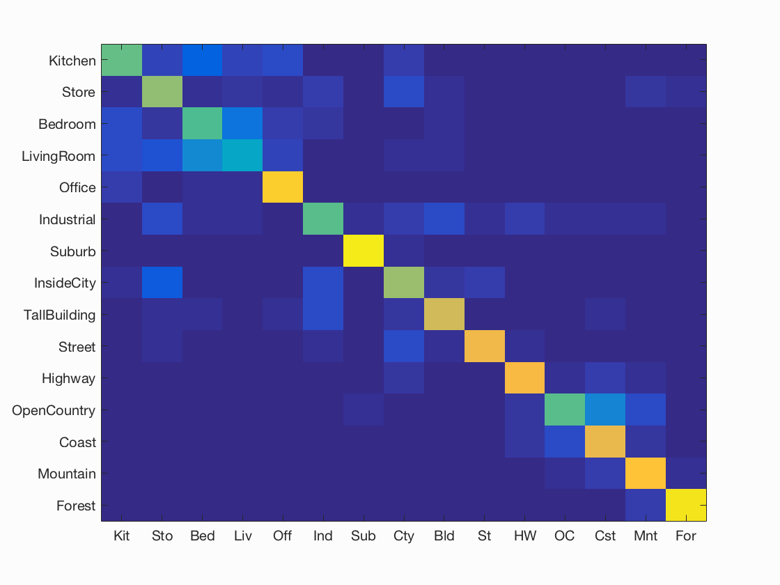
Accuracy (mean of diagonal of confusion matrix) is 0.712
| Category name | Accuracy | Sample training images | Sample true positives | False positives with true label | False negatives with wrong predicted label | ||||
|---|---|---|---|---|---|---|---|---|---|
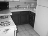
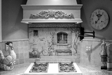
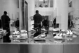
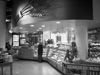
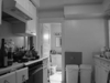
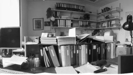
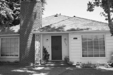
| Kitchen | 0.570 |  |
 |
 |
 |
 Bedroom |
 LivingRoom |
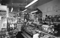
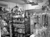
 Store |
 Store |
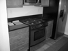
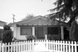
| Store | 0.630 | 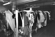 |
 |
 |
 |
 LivingRoom |
 LivingRoom |
 Kitchen |
 Street |
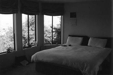
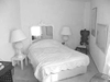
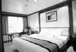
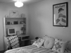
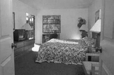
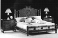
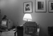
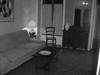
| Bedroom | 0.540 | 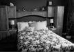 |
 |
 |
 |
 Store |
 Kitchen |
 Kitchen |
 Industrial |
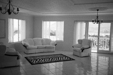
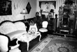
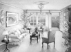
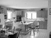
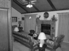
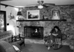
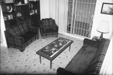
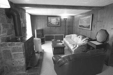
| LivingRoom | 0.390 |  |
 |
 |
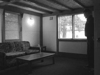 |
 InsideCity |
 Bedroom |
 Bedroom |
 Store |
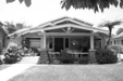
| Office | 0.890 |  |
 |
 |
 |
 Kitchen |
 Bedroom |
 Suburb |
 LivingRoom |
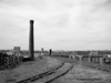
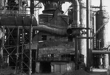
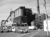
| Industrial | 0.550 | 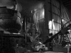 |
 |
 |
 |
 Highway |
 Bedroom |
 InsideCity |
 TallBuilding |
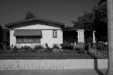
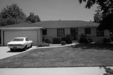
| Suburb | 0.960 | 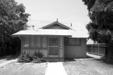 |
 |
 |
 |
 Mountain |
 Industrial |
 InsideCity |
 Store |
| InsideCity | 0.650 |  |
 |
 |
 |
 TallBuilding |
 Kitchen |
 Store |
 Store |
| TallBuilding | 0.740 |  |
 |
 |
 |
 LivingRoom |
 Mountain |
 Industrial |
 Office |
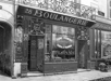
| Street | 0.800 |  |
 |
 |
 |
 Industrial |
 OpenCountry |
 Highway |
 Industrial |
| Highway | 0.820 |  |
 |
 |
 |
 Store |
Street |
 Mountain |
 Coast |
| OpenCountry | 0.560 |  |
 |
 |
 |
 Coast |
 Highway |
 Coast |
 Coast |
| Coast | 0.790 |  |
 |
 |
 |
 Mountain |
 Highway |
 Highway |
 OpenCountry |
| Mountain | 0.850 |  |
 |
 |
 |
 OpenCountry |
 Forest |
 Coast |
 LivingRoom |
| Forest | 0.940 |  |
 |
 |
 |
 Mountain |
 Store |
 Mountain |
 Store |
The trend of the vocab is fairly intuitive. As it increases, the classification accuracy increases as well until around 400, where it levels out. The time increases as well, being especially prohibitive at around 600 words. Going with something around 200 gives the best tradeoff between time and accuracy.
Effect of Vocab Size
| Vocabulary Size | 10 | 50 | 100 | 200 | 400 | 600 | 1200 |
| Classification Accuracy | 38% | 61% | 66% | 68% | 71% | 71% | 72% |
| Time | 8 min | 9 min | 10 min | 11 min | 14 min | 20 min | 30 Min |
The value of K has some effect on the accuracy, giving a boost of a few points. But it's nothing particulary significant.
Best Classification Results with K Nearest Neighbors
| K with 400 Vocab Size | 1 | 5 | 15 | 30 | 50 |
| Classification Accuracy | 51% | 53% | 53% | 50% | 49% |
Hyper-Parameters
These are the values I used to get the fastest results.- Vocab Size - this was addressed above. The accuracy steadily increased until 400, where it leveled off.
- Pyramid Size and Sigma - To get SIFT features at different scales, the images are blurred and resized. To keep the time to a minimum, I only used 4 different scales. I used a sigma of 2.0. When I raised the value to 4, this decreased the accuracy by around a point.
- Step Size - the value specified is the horizontal and vertical displacement of each feature center to the next. This serves as the sampling density. The value of 10 seemed to give the best results when generating the vocab, and a smaller more fine grained value of 5 worked for particular images. I tried 15 for both, but this seemd to reduce the accuracy by a few points.
- SIFT Feature Size - I used the standard 4x4 size SIFT features.
- Sample Size - this parameter dictated what percentage of the features of an image were used to when generating the vocab words. I used 0.8, as this sped things up slightly without sacrificing performance.
- Binning size and weights - these parameters dictated how a specific feature of an image contributes to an image histogram. I took the top five matches, thus 5 bins, and weighted the closest match with 1.0, the second with 0.5, the third with 0.025, the fourth with 0.0125, and the fifth weight was 0.00625. This served as an easy way to increase accuracy; frankly, I didn't mess around with these values too much, as they seemed reasonable and experimentation took 5-10 minutes each time.
- Regularization - I tried values from 0.00001 all the way up to 1.0. The accuracy went from 59% to 73% back to 62%. The best value was 0.0006.
- K in the K Nearest Neighbor - this was addressed above. The best K value was around 30.