Project 4 / Scene Recognition with Bag of Words
In this project I performed scene recognition using a trained classifier on 15 different types of scenes. Scene recognition using the bag of words model first consists of creating a vocabulary of SIFT features from every training image. Test images are then given a feature representation based on the distance of its features to each of to the vocabulary words. The test image representations are passed into a classifer, and assigned a label, the type of scene in this case.
This project tested three different combinations of feature representations and classifiers:
- Tiny image features and k-NN classifier
- Bag of SIFT features and k-NN classifier
- Bag of SIFT features and linear SVM classifier
1: Tiny Image Features and K-NN Classifier
Tiny image features were constructed by resizing each image to a 16x16 image, flattening to a 1x256 vector, and normalized to unit length. These features were then passed into a k-NN classifier (k=5), which returns the label of the image with the closest Euclidian distance. The entire pipeline took 1:24 and resulted in the highest accuracy of 19.3%.
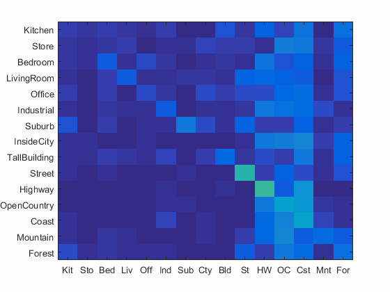
Confusion matrix. Mean accuracy = 0.193
2: Bag of SIFT Features and K-NN Classifier
To classify images with the bag-of-words model, a vocabulary was first built. For every input image, SIFT features were sampled (10 each) to produce a list of ~15000 total features. To create a vocabulary of features from these samples, k-means was run (k=100), to find the 100 centers, or vocabulary words to represent future images.
After creating the vocabulary, SIFT features were extracted from both testing and training images. These SIFT features were sampled (25%), and the distances to each of the vocabulary words was computed. Using this information, a histogram of votes to the closest vocabulary word was created for each image. This histogram was then and normalized into a 1x100 vector representation.
Again, the same k-NN (k=5) algorithm was run to classify the test images, which resulted in 50.9% accuracy. The runtime was 2:25.
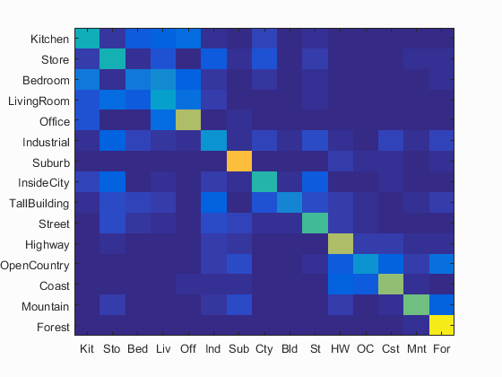
Confusion matrix. Mean accuracy = 0.509
3. Bag of SIFT Features and Linear SVM Classifier
Using the same process above, a bag-of-words feature representation was created for each image. The images were then pased into an SVM classifier.
An one vs. all SVM classifier was created for every scene label (15) and trained on the input images with lambda=0.0001. The resulting classifiers were used to score each test image for its distance. The highest scoring classifier for each image was used to label the image. Results reached 63.4% mean accuracy. The runtime was 2:15.
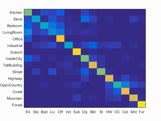
Confusion matrix. Mean accuracy = 0.634
| Category name | Accuracy | Sample training images | Sample true positives | False positives with true label | False negatives with wrong predicted label | ||||
|---|---|---|---|---|---|---|---|---|---|
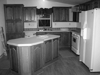
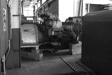
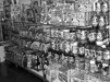
| Kitchen | 0.600 |  |
 |
 |
 |
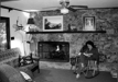
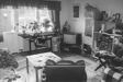
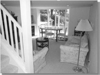
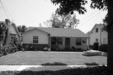
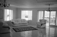
 LivingRoom |
 InsideCity |
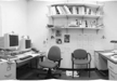
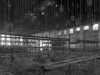
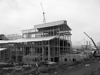
 Office |
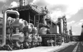
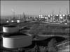
 Industrial |
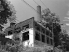
| Store | 0.360 | 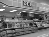 |
 |
 |
 |
 Industrial |
 Kitchen |
 LivingRoom |
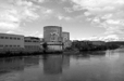
 Coast |
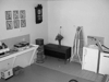
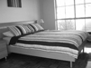
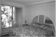
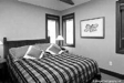
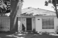
| Bedroom | 0.400 |  |
 |
 |
 |
 InsideCity |
 LivingRoom |
 Industrial |
 Kitchen |
| LivingRoom | 0.270 | 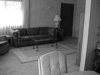 |
 |
 |
 |
 Street |
 Office |
 Kitchen |
 Office |
| Office | 0.850 |  |
 |
 |
 |
LivingRoom |
 Kitchen |
 Kitchen |
 Suburb |
| Industrial | 0.370 | 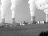 |
 |
 |
 |
 TallBuilding |
 TallBuilding |
 Mountain |
 Kitchen |
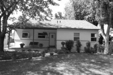
| Suburb | 0.920 | 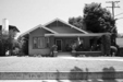 |
 |
 |
 |
 Mountain |
 Mountain |
 TallBuilding |
 InsideCity |
| InsideCity | 0.600 |  |
 |
 |
 |
 Store |
 LivingRoom |
 Kitchen |
 TallBuilding |
| TallBuilding | 0.770 |  |
 |
 |
 |
 Industrial |
 Mountain |
 Kitchen |
Industrial |
| Street | 0.610 |  |
 |
 |
 |
 TallBuilding |
 Industrial |
 InsideCity |
 Highway |
| Highway | 0.780 |  |
 |
 |
 |
 Industrial |
 OpenCountry |
 Coast |
 Coast |
| OpenCountry | 0.470 |  |
 |
 |
 |
 Coast |
 Mountain |
 Highway |
 Coast |
| Coast | 0.800 |  |
 |
 |
 |
 OpenCountry |
 OpenCountry |
 OpenCountry |
 OpenCountry |
| Mountain | 0.760 |  |
 |
 |
 |
 Store |
 Forest |
 OpenCountry |
 OpenCountry |
| Forest | 0.950 |  |
 |
 |
 |
 Store |
 Mountain |
 Mountain |
 TallBuilding |
| Category name | Accuracy | Sample training images | Sample true positives | False positives with true label | False negatives with wrong predicted label | ||||