Project 4 / Scene Recognition with Bag of Words

Overview

For this project, I used three combinations of techniques to match images to labels given a training set of (image, label) pairs. I achieved the most accurate classification (68.4%) with bags of SIFT combined with linear SVMs.

Tiny images and Nearest Neighbor

The first technique I used for classification was using tiny versions of the original images as features and then nearest neighbor to classify test cases. I chose to use 16x16 as my tiny image resolution. For a given test image, Nearest Neighbor looks for the training image whose tiny image is closest to the tiny image of the test image. The label of the closest training image is then outputted for the test image.

Results

For this results section and the next two results sections, accuracy refers to the mean of the diagonal of the confusion matrix. I achieved a classification accuracy of 19.1% with this method of classification.

Bag of SIFT and Nearest Neighbor

The second technique I tried was using a Bag of SIFT features to represent the images, but still using nearest neighbor to classify test cases. Creating bags of SIFT features was done as follows. First a vocabulary of SIFT features is built from the test set by sampling SIFT features from the training images and then clustering the sampled features using kmeans clustering for some k. I found that the best number of clusters for me, aka my vocab size, was 250. Any vocab size larger than this took longer to run without much payoff in accuracy. I found that a step size of 10 was fast and gave accurate results when detecting these initial SIFT features to build the vocabulary. I took 200 SIFT features from each image when building a vocabulary. Next, for each test image, SIFT features were calculated and placed in a bin corresponding to the closest cluster center from the vocabulary. I found that a step size of 5 was fairly fast and accurate when detecting SIFT features in this step. The bags of SIFT are normalized so that varying images sizes don't affect results by producing more or less SIFT features. For the fast-running, less-accurate version of the code specified in the "Guidelines for Project 4" on Piazza, I changed to step size to 10 for this step.

My SIFT binning and normalization code looks like this:

% put them in bins
bins = zeros(1, vocab_size);
SIFT_features = SIFT_features';
dists = vl_alldist2(single(SIFT_features'), single(vocab'));
for i = 1:size(SIFT_features, 1)
	dist_row = dists(i, :);
	[~, min_index] = min(dist_row);
	bins(1, min_index) = bins(1, min_index) + 1; %increment proper bin in histogram
end
%normalize histogram
bins = bins ./ sum(bins);

Results

Accuracy was greatly increased with this method to 50.8% at a step size of 5 for SIFT feature detection as mentioned above and 48.4% accuracy with a step size of 10.

Bag of SIFT and Linear SVM

Next, I kept the bags of SIFT and replaced the nearest neighbor classifier with a 1 v all SVM classifier. For each category, I trained an SVM to classify images as either in that category or not. To choose a category for a test image, I took the label of the SVM with the highest confidence. I found that a LAMBDA of .000001 provided the best classification accuracy with an SVM classifier. I kept my bags of SIFT feature detection step size at 5 for the slow version/more-accurate version of the code and 10 for the fast version that we are required to submit.

SVMS are trained as follows:

for category_index = 1:num_categories
    matching_indices = strcmp(categories{category_index, 1}, train_labels);
    matching_indices = double(matching_indices); %gets rid of some complaint that svmtrain() has
    matching_indices(matching_indices == 0) = -1; %convert zeros to negative ones which svmtrain() requires
    binary_labels = matching_indices';
    LAMBDA = .000001;
    [W B] = vl_svmtrain(train_image_feats', binary_labels, LAMBDA);
    % save for later evaluation of test cases
    % there is a column for each category
    w_s = [w_s W];
    b_s = [b_s B];
end

And confidences are evaluated for each test image like so:

predicted_categories = cell(size(test_image_feats, 1), 1);
for i = 1:size(test_image_feats, 1)
    test_image_feat = test_image_feats(i, :);
    confidences = w_s' * test_image_feat' + b_s';
    [~, max_index] = max(confidences); % get the index of max confidence
    predicted_categories{i, 1} = categories{max_index, 1};
end

Results

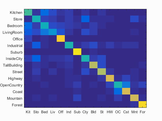
The overall accuracy and accuracies for each label are displayed below. Note that some categories achieved much higher accuracy than others. With a step size of 5 on SIFT feature detection for bags of SIFT, accuracy was 68.4%. With a step size of 10, it was 63% accurate.

Scene classification results visualization

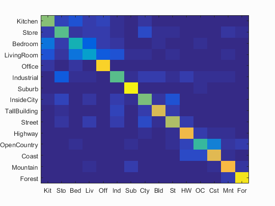
Accuracy (mean of diagonal of confusion matrix) is 0.684

Category name	Accuracy	Sample training images		Sample true positives		False positives with true label		False negatives with wrong predicted label
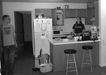
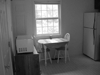
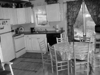
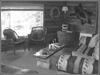
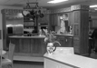
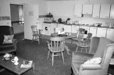
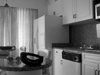
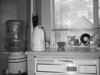
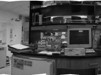
Kitchen	0.610		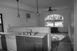			Bedroom	Office	Store	TallBuilding
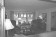
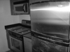
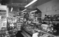
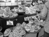
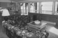
Store	0.550					LivingRoom	Industrial	Bedroom	Highway
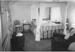
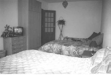
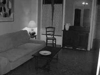
Bedroom	0.450					LivingRoom	LivingRoom	Industrial	LivingRoom
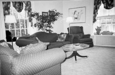
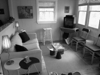
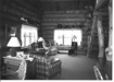
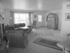
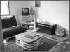
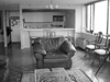
LivingRoom	0.350		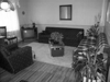			InsideCity	InsideCity	InsideCity	Bedroom
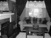
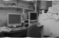
Office	0.900					LivingRoom	LivingRoom	Kitchen	Kitchen
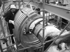
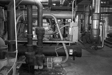
Industrial	0.550					Store	OpenCountry	Store	Highway
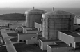
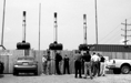
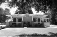
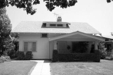
Suburb	0.970		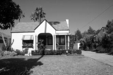			LivingRoom	Mountain	OpenCountry	InsideCity
InsideCity	0.600					Highway	Kitchen	Store	Street
TallBuilding	0.750					Bedroom	InsideCity	InsideCity	InsideCity
Street	0.680					Store	InsideCity	Store	LivingRoom
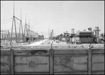
Highway	0.810					OpenCountry	Industrial	Forest	OpenCountry
OpenCountry	0.510					Coast	TallBuilding	Coast	Coast
Coast	0.770					OpenCountry	OpenCountry	OpenCountry	Highway
Mountain	0.820					Forest	TallBuilding	LivingRoom	TallBuilding
Forest	0.940					TallBuilding	OpenCountry	Mountain	Mountain
Category name	Accuracy	Sample training images		Sample true positives		False positives with true label		False negatives with wrong predicted label

Here are the results for the fast version of the code with bigger SIFT step size when finding bags of SIFT.

Scene classification results visualization

Accuracy (mean of diagonal of confusion matrix) is 0.630

Category name	Accuracy	Sample training images		Sample true positives		False positives with true label		False negatives with wrong predicted label
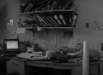
Kitchen	0.520		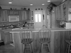			Office	LivingRoom	LivingRoom	InsideCity
Store	0.440					TallBuilding	Street	LivingRoom	InsideCity
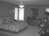
Bedroom	0.430		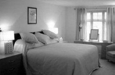			Store	LivingRoom	LivingRoom	Kitchen
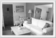
LivingRoom	0.310					Kitchen	Kitchen	Office	Kitchen
Office	0.880		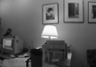			Bedroom	Kitchen	LivingRoom	Bedroom
Industrial	0.460					TallBuilding	InsideCity	Coast	Kitchen
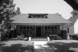
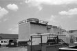
Suburb	0.940		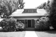			Industrial	Highway	LivingRoom	Street
InsideCity	0.460					Store	Industrial	Store	Kitchen
TallBuilding	0.700					LivingRoom	LivingRoom	Store	Street
Street	0.680					TallBuilding	Kitchen	TallBuilding	Highway
Highway	0.760					Store	Store	Coast	Street
OpenCountry	0.460					Bedroom	Mountain	Forest	Forest
Coast	0.760					TallBuilding	OpenCountry	Suburb	OpenCountry
Mountain	0.740					TallBuilding	Store	TallBuilding	OpenCountry
Forest	0.910					OpenCountry	Store	Street	Mountain
Category name	Accuracy	Sample training images		Sample true positives		False positives with true label		False negatives with wrong predicted label