Michael Avidano

Project 4: Scene Recognition with Bag of Words

Overview

The main goal of this project was the classification of various images into generic "categories". To do this task, a set of training images with known categories were broken down into key features. Testing images were then broken down in the same way. One of two classifiers was used to match the features from test images to those from training images, and a specific category was assigned to each image.

In both the feature extraction and the classification tasks, two different methods were used. For features methods, the "tiny image" feature and the "bag of SIFT" feature were used. For classifiers, a nearest neighbor classifier and a singular value matrix (SVM) classifier were used.

Feature Extraction: Tiny Image

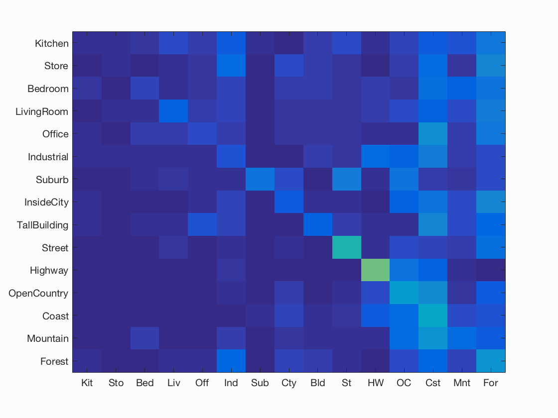
The idea behind the tiny image feature is that a normalized "small" image will have similarities across the same category and require very little processing power to create. Each image was shrunk to a 16x16 image, then the image was normalized and resized into a single row. When resizing non-square images, the image was cropped to a square at the center of the image, then the standard downsizing process was done. The general performance of this feature was poor, with only 20% accuracy over the 15 categories, but outperformed random chance.

Feature Extraction: Bag of SIFTs

Bag of SIFTs feature assignment is based on the categorization of SIFT features into visual words. For this feature method, first a vocabulary of visual words is constructed. The vocabulary was constructed by taking a sample of 20,000 SIFT features and clustering them using the K-means algorithm explored in class. Then, a histogram was constructed for each image that listed all of the occurrences of various visual words within the image. This histogram was normalized and used to classify all further images.

Classification: Nearest Neighbor

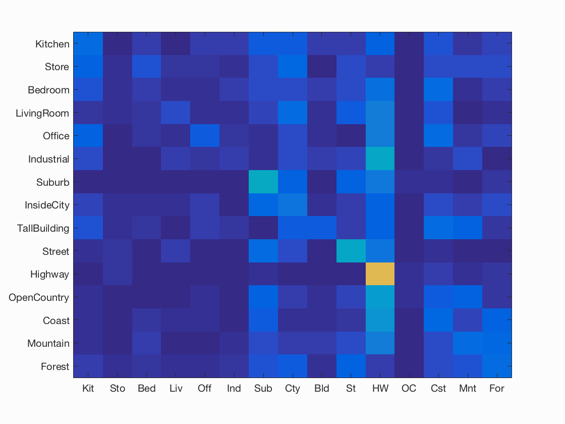
When classifing each test image, the basic nearest neighbor algorithm simply chooses the training image with the minimum differences from the test image. I used a slightly different algorithm, choosing the 10 closest matches, then weighting each choice based on its distance away. The net closest category was then assigned as the test image category. Additionally, the distance method calculation used was changed based on the feature used: tiny images used standard distance calculations, whereas bag of SIFT features used chi-squared distance calcualtions. The basic code for this selection is shown below.

k = 10; % Number of closest matches selected for comparison
for j = 1:c
% get k closest match labels
    labelNums = [];
    for label = train_labels(locArr(1:k,j))'
        labelNums(end+1) = find(strcmp(allLabelTypes,label));
    end
    % Assign weight to each match as inverse of distance
    weights = 1 ./ distArr(1:k,j)';

    % Sum the weights based on label
    weightedLabels = zeros(length(allLabelTypes),1);
    for i = 1:length(weights)
        weightedLabels(labelNums(i)) = weightedLabels(labelNums(i)) + weights(i);
    end

    % Highest weighted label becomes assigned label
    [~,loc] = max(weightedLabels);
    predicted_categories(j) = allLabelTypes(loc);
end

Classification: Singular Value Matrix (SVM)

The other classifier used was a singular value matrix method. For this method, a hyperplane was constructed based on the training images, and the parameters are then recorded. These parameters represent a linear singular value matrix that was then used to quickly categorize all of the test images. In creating the SVM, one of the free parameters is the value of lambda. A series of tests were carried out to calculate the best lambda value, with the results recorded below.

Analysis of Lambda Value for SVM

Lambda Value	0.0001	0.001	0.01	0.1	1	10	100
Mean Accuracy	0.525	0.527	0.526	0.573	0.600	0.555	0.476
Standard Deviation	0.0100	0.0098	0.0105	0.0031	0.0046	0.0110	0.0202

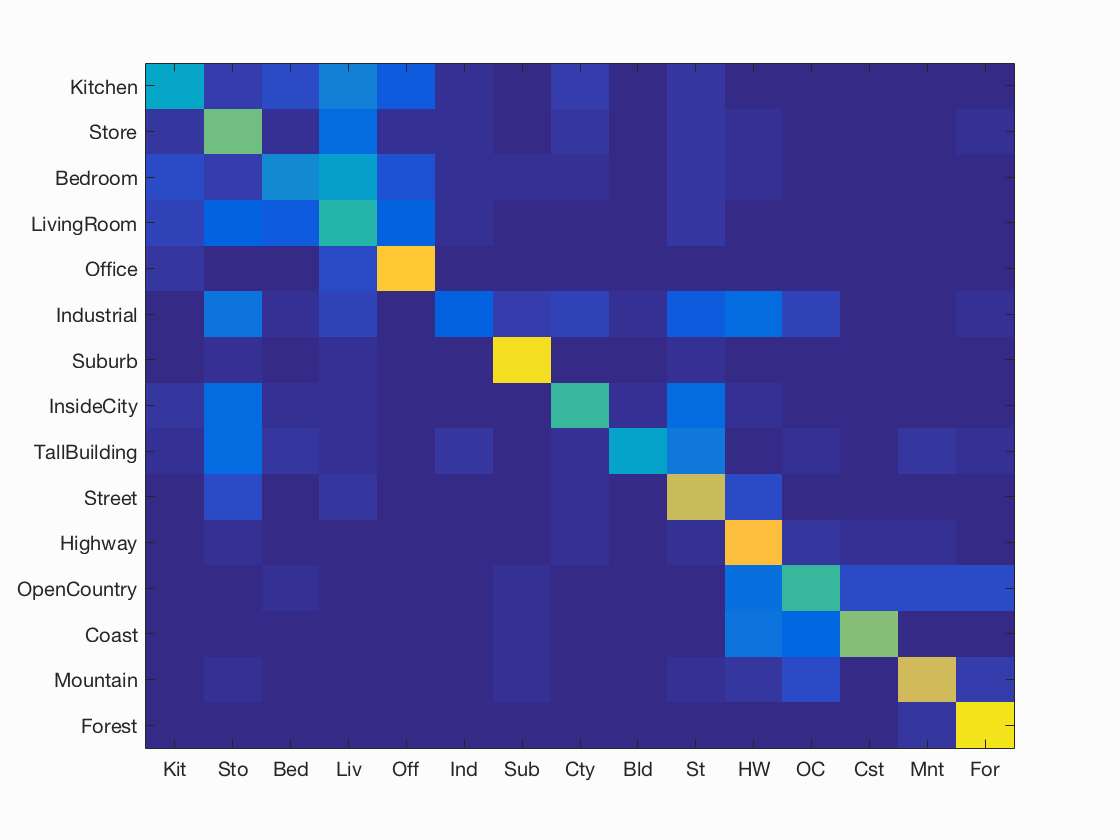
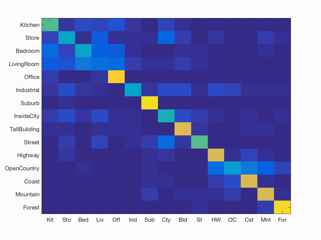
For each lambda value, 100 iterations of the SVM were constructed, and the average accuracy and standard deviation are given above. The best lambda value was found to be approximately 1. This classifier showed very slight improvement over the nearest neighbor classifier for bag of SIFTs, but the improvement was not significant.

Performance